
Zome Primer
Zome Primer
Elements of Zonohedra Geometry
Steve Baer
Zomeworks Corporation | Albuquerque, New Mexico
ISBN: 978-000000000-0
ISBN-10: 0
Updated: 2024-12-15
To
My Wife Holly
Preface
This booklet has first an elementary explanation of the geometry of Zonohedra, then a more difficult account of the growths of the thirty-one zone star. This system, based on the 31 lines that pass through the center of an icosahedron and either a vertex, edge midpoint or face midpoint is new and unusual.
I have applied for a patent on this structural system. The patent is assigned to Zomeworks Corporation. The predecessors of this system are the octet truss and the MERO space grid system. The relative potentials of these systems are discussed briefly by a comparison of their geometric possibilities.
The forms possible using this system are limitless; there is no attempt here to explore these possibilitiesthe examples shown are small probings. The booklet describes the mathematics of the process that creates these limitless forms.
The framework for the Robert Ford residence was designed by Jim Welty and Robert Ford.
The shallow rectangular based trusses were designed by Berry Hickman of Zomeworks who also introduced the excellent plastic ball joint used throughout in the models photographed.
The design and manufacture of the 6-zone aluminum joint was done by Otto Jung of Design Industries in Albuquerque.
Ken Leonard did the layout and both he and my wife, Holly, gave much editorial assistance.
S.C.B.
Albuquerque
August 1970
Zomes, Domes and Clusters
What Are Zomes?
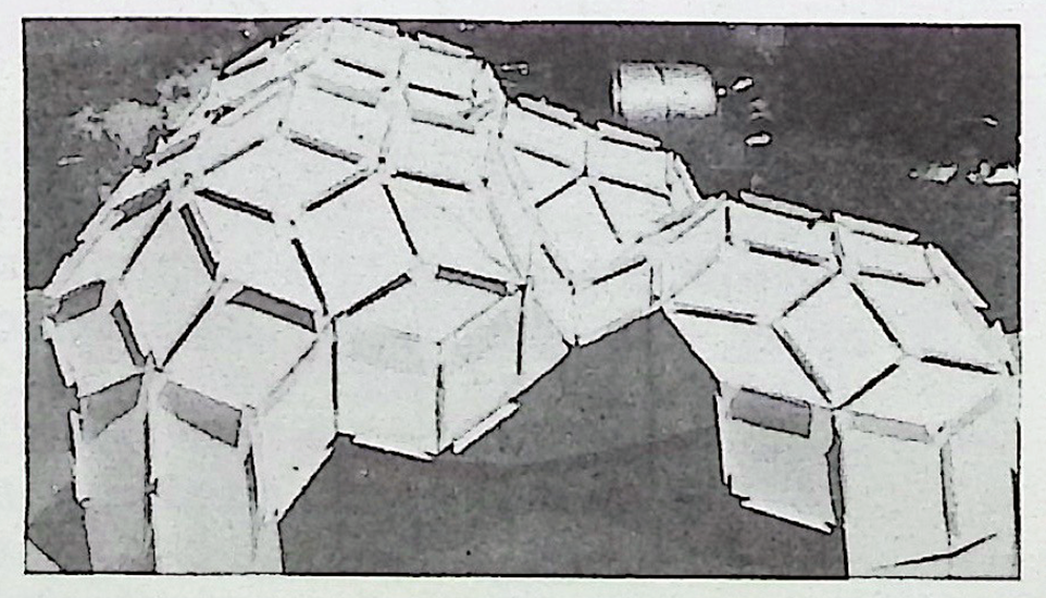
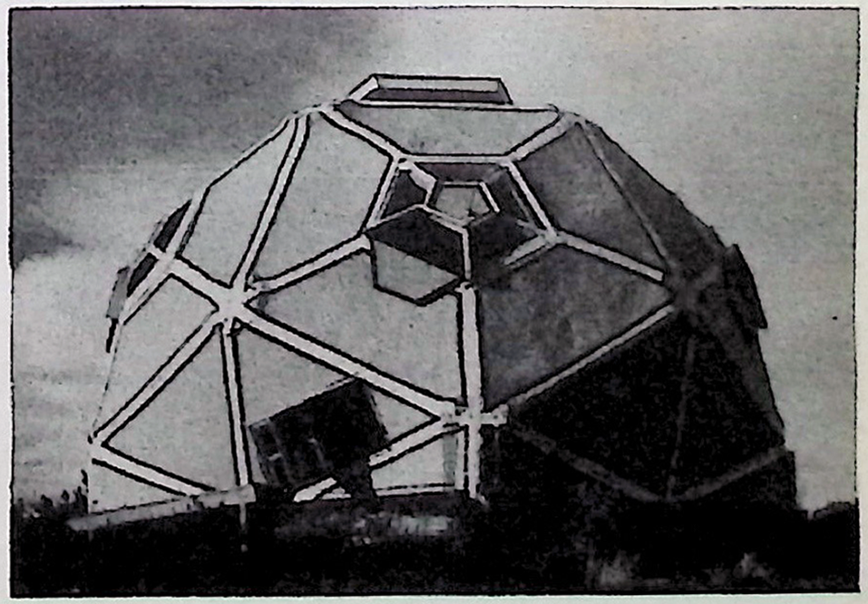
A Zome is a man-made structure derived from zonohedra. The zones of the zonohedron may be stretched or shrunk or removed to produce, if desired, an asymmetric dome shaped structure.
Zomes may be single or clustered.
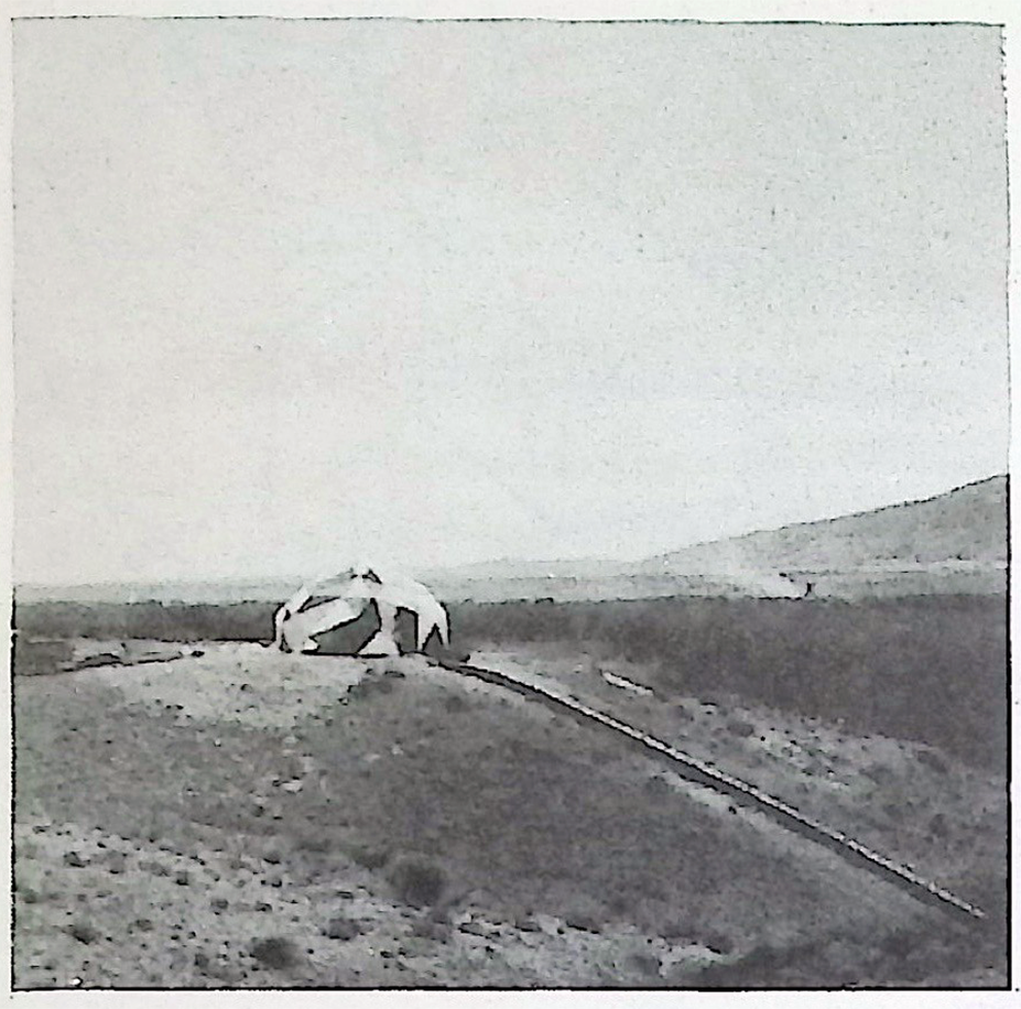
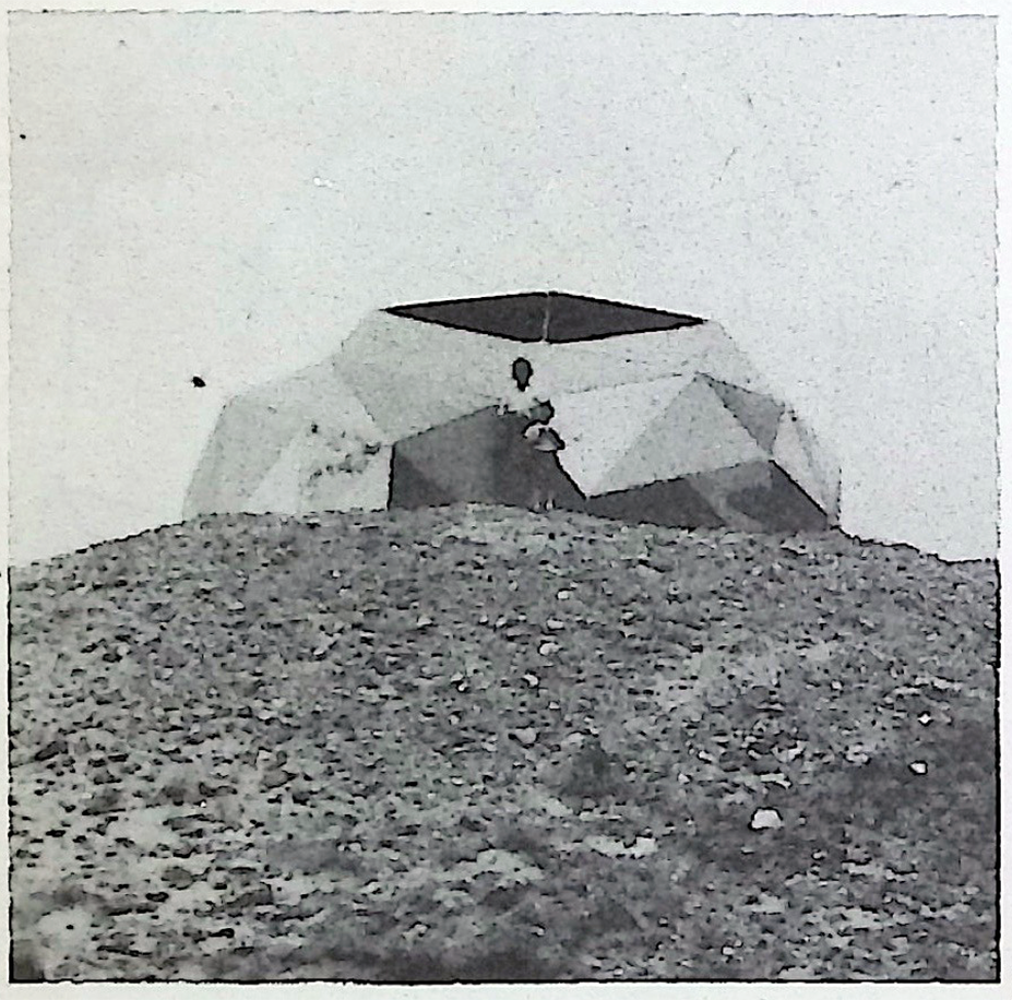
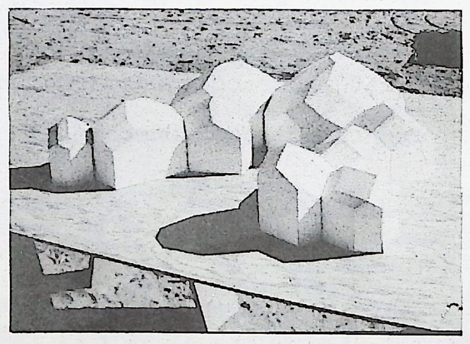
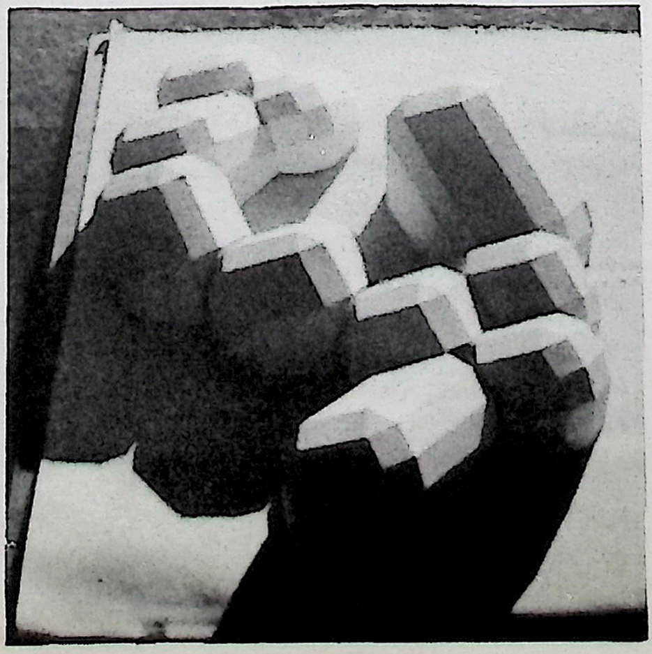
Zomes can cluster together like soap bubbles. Their zones can be stretched, shrunk, or omitted completely to make the various zomes’ different shapes and sizes. The zomes can also pack several layers deep.
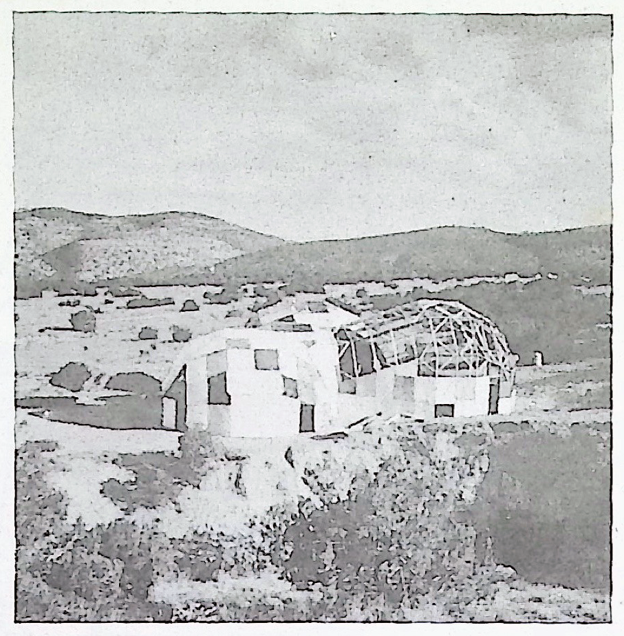
What is the Difference Between a Zome and a Geodesic Dome?
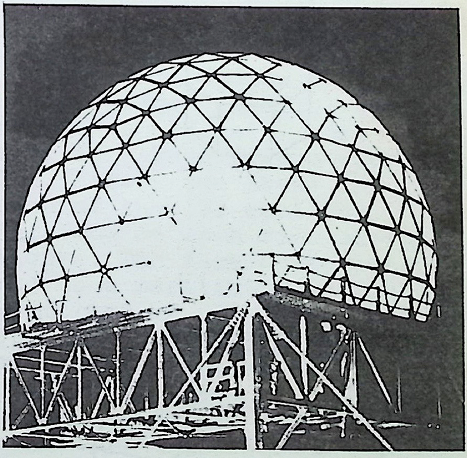
A geodesic dome is a structure which closely follows the shape of the sphere and whose edge lengths closely follow the path of great circles on the sphere. (These are the sphere’s geodesics.) The geodesic dome, because of its shape, and the arrangement of its structural members is extremely strong, but its uses are limited because of the inflexibility of its shape. It is always part of a sphere—a low bubble or a high bubble—its floor is always a circle—any variation would destroy the structural properties of the geodesic dome. The geodesic dome, if it is large and composed of many edges and joints, has many different edge lengths. It is complicated in structure and simple in shape. Zomes are simple in structure and complicated in shape.
Zonohedra
What are Zonohedra?
A zonohedron is a convex solid, all of whose faces are polygons with edges in equal and parallel pairs.
These are possible faces for zonohedra:
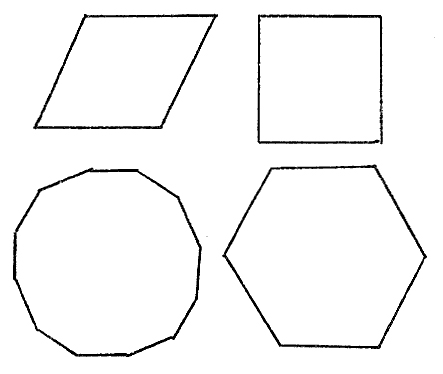
These are zonohedra:
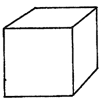
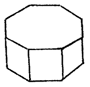
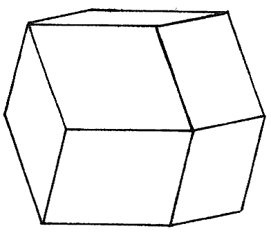
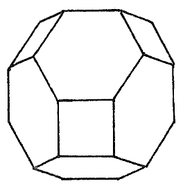
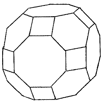
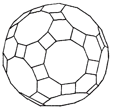
A zone of edges is a band of parallel edges which circles the solid. Every edge belongs to a zone.
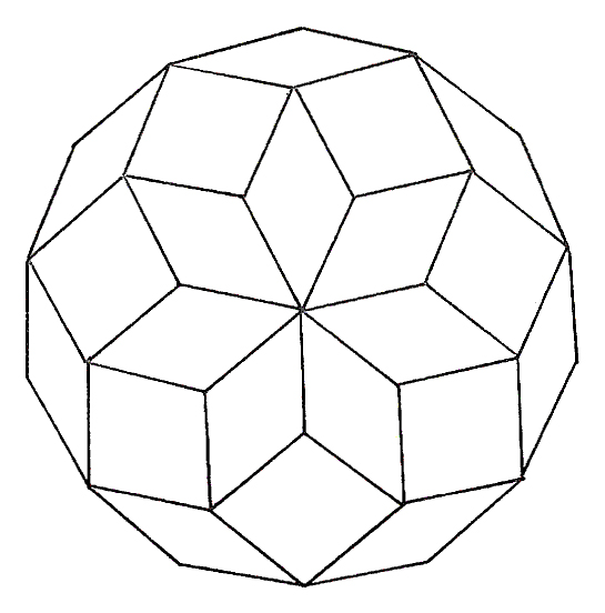
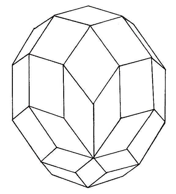
Face Planes of Zonohedra
A plane is defined by two lines. A six-zone figure has six different lines; 1, 2, 3, 4, 5, 6. How many pairs can we form with six objects?
| 1,2 | 2,3 | 3,4 | 4,5 | 5,6 | |
| 1,3 | 2,4 | 3,5 | 4,6 | ||
| 1,4 | 2,5 | 3,6 | = 15 | ||
| 1,5 | 2,6 | ||||
| 1,6 |
: Pairs of Six Objects
Algebraic expression:
X = \frac{(n)(n-1)}{2}
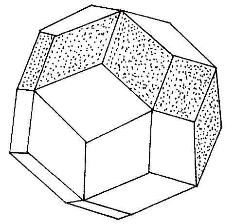
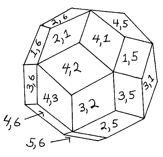
Rhombic Triacontahedron with face planes labeled with numbers of the zones which form the plane.
There are then 15 more faces on the other side which add up to the 30 faces of the Triacontahedron.
The ten-zone system can form
This figure is the enneacontahedron with its faces marked:
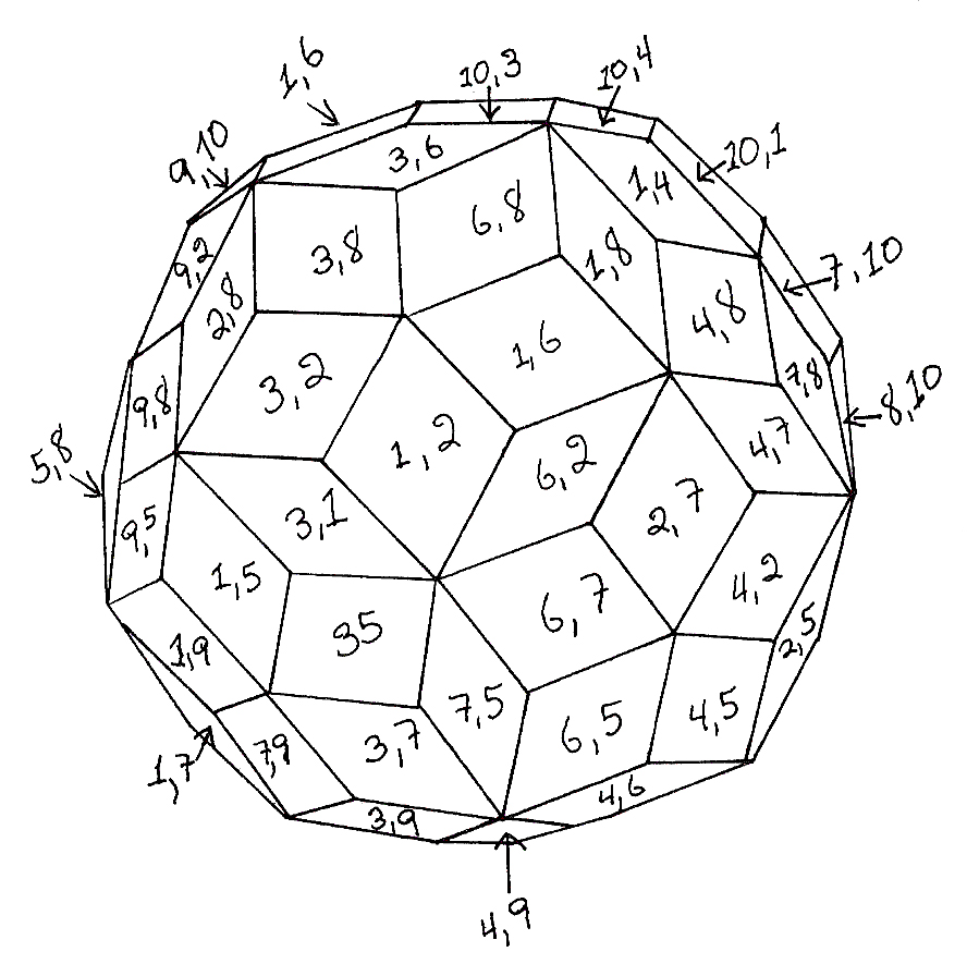
The equation is for the number of planes, and if we wish to find the total number of faces for the polyhedron, including the back side, multiply the number of different planes by 2, and this equals
The formula
If three lines of the star lie in one plane, then the zonohedron associated with the star has a pair of hexagons. If more than three lines lie in one plane, then there are facets to the zonohedron with corresponding more edgesoctagon, decagon, etc.
Section Stars and Face Planes
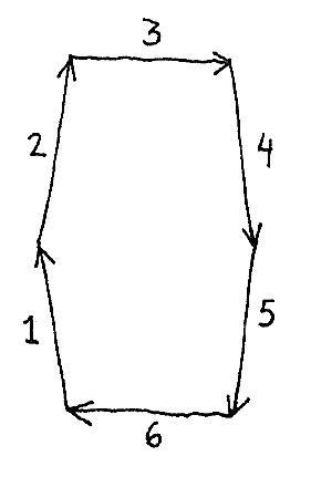
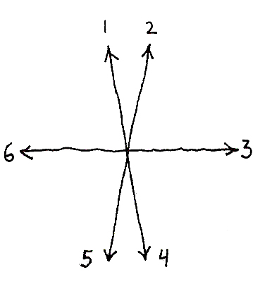
The zonohedron that has its edges parallel with the lines of the 31-zone star is a huge figure with facestwo faces for each of the 121 sections one face on each side of the figure. The face corresponding to a particular section is formed by the lines of the star following each other head to toe around in a complete polygon. Consequently, the 242 sided zonohedron associated with the 31 zone star has:
| regular decagons | T sections | |
| irregular dodecagons | R sections | |
| irregular hexagons | S sections | |
| regular hexagons | V sections | |
| rectangles | X sections | |
| rectangles | Y sections | |
: Faces of a 31 Zone Star
Division of Zonohedra into Parallepiped Cells
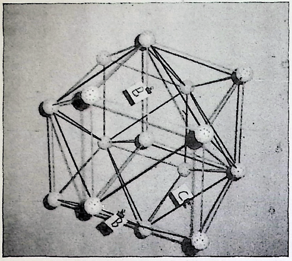
Every zonohedron can be divided into component parallelepiped cells. Every set of three different lines form one cell. In the case of the four-zone rhombic dodecahedron 2.17, there are then:
C_{3}^{4}= \dfrac{4\cdot3\cdot2}{3\cdot2\cdot1}= 4\ \text{cells.}\label{eq:c_3_4}
The sides of the component parallelepiped cells are necessarily the same as the sides of the complete figure.
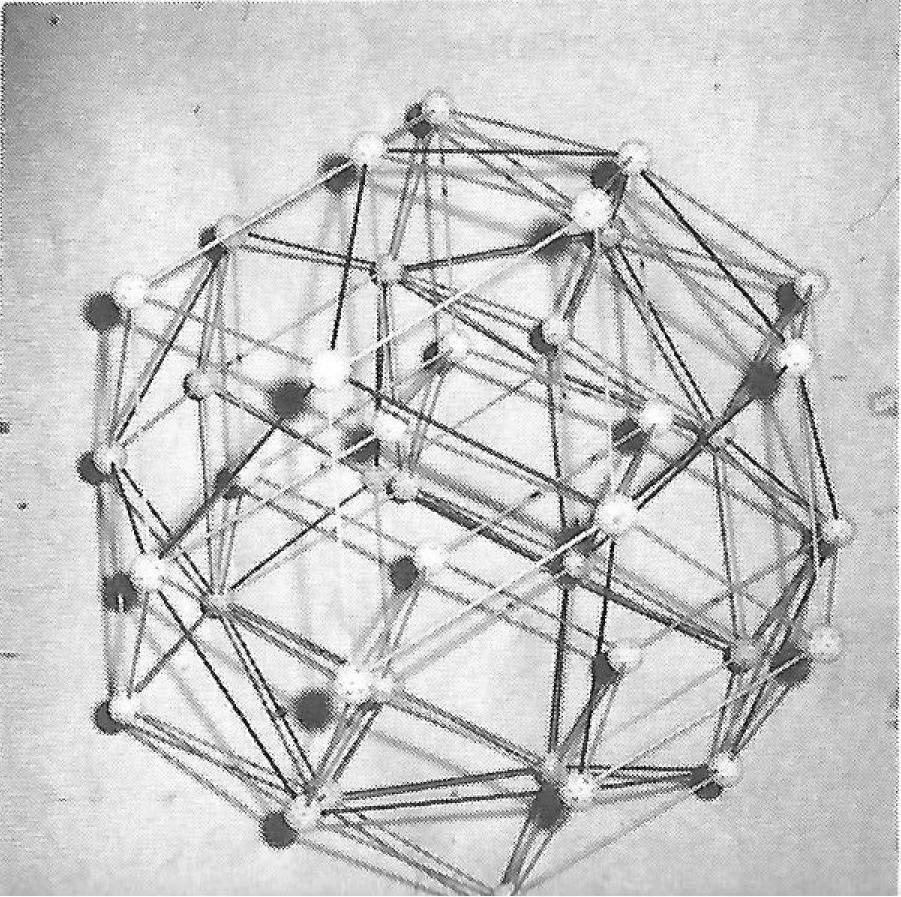
The triacontahedron subdivides into:
C_{3}^{6}= \dfrac{6\cdot5\cdot4}{3\cdot2\cdot1}= 20\ \text{cells.}\label{eq:c_3_6}
The rhombic triacontahedron divides into 10 acute and 10 obtuse parallelepipeds.
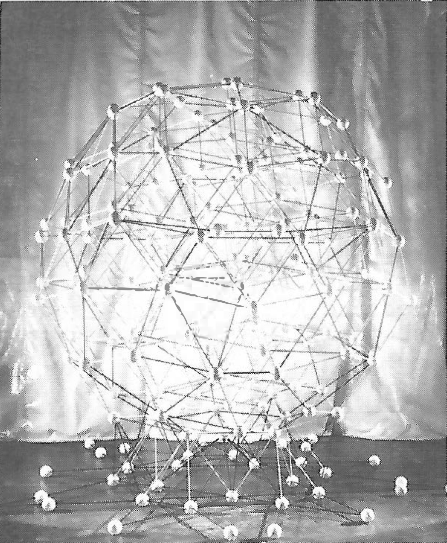
The enneacontahedron subdivides into ```block-katex
C_^= \dfrac= 120\ \text\label
There are five different kinds of cells. With one kind of diamond, there are only two kinds of cells possible, but the enneacontahedron has two kinds of diamond faces allowing for more types of cells.

There are:

|                  |         |                   |                   |        |
|-----------------:|--------:|:------------------|:------------------|:-------|
|             $`10`$ | A cells | 6 fat diamonds    |                   | acute  |
|             $`20`$ | B cells | 6 fat diamonds    |                   | obtuse |
|             $`30`$ | C cells | 4 fat diamonds    | 2 skinny diamonds | acute  |
|             $`30`$ | D cells | 4 skinny diamonds | 2 fat diamonds    | acute  |
|             $`30`$ | E cells | 2 skinny diamonds | 4 fat diamonds    | obtuse |
| $`\overline{120}`$ |   cells |                   |                   |        |

: Cells of the Enneacontahedron

# Regular Ways of Arranging Lines in Space

The regular polyhedra are like seeds from which growths may appear. They are the connecting joints for the zonohedra. The joints are all parallel to each other. The lines of the zonohedra are perpendicular to the faces of the joints.

## Three Zones

<figure id="fig:28">
<img src="content/images/fig-28.jpg" alt="Figure 28: Cube" />
<figcaption aria-hidden="true">Figure 28: Cube</figcaption>
</figure>

## Four Zones

<figure id="fig:29">
<img src="content/images/fig-29.jpg" alt="Figure 29: Tetrahedron" />
<figcaption aria-hidden="true">Figure 29: Tetrahedron</figcaption>
</figure>

<figure id="fig:30">
<img src="content/images/fig-30.jpg" alt="Figure 30: Octahedron" />
<figcaption aria-hidden="true">Figure 30: Octahedron</figcaption>
</figure>

<figure id="fig:31">
<img src="content/images/fig-31.jpg" alt="Figure 31: Rhombic Dodecahedron" />
<figcaption aria-hidden="true">Figure 31: Rhombic Dodecahedron</figcaption>
</figure>

## Six Zones

<figure id="fig:32">
<img src="content/images/fig-32.jpg" alt="Figure 32: Dodecahedron" />
<figcaption aria-hidden="true">Figure 32: Dodecahedron</figcaption>
</figure>

<figure id="fig:33">
<img src="content/images/fig-33.jpg" alt="Figure 33: Rhombic Triacontahedron" />
<figcaption aria-hidden="true">Figure 33: Rhombic Triacontahedron</figcaption>
</figure>

## Ten Zones

<figure id="fig:34">
<img src="content/images/fig-34.jpg" alt="Figure 34: Icosahedron" />
<figcaption aria-hidden="true">Figure 34: Icosahedron</figcaption>
</figure>

<figure id="fig:35">
<img src="content/images/fig-35.jpg" alt="Figure 35: Rhombic Enneacontahedron" />
<figcaption aria-hidden="true">Figure 35: Rhombic Enneacontahedron</figcaption>
</figure>

# Clustering

## Twenty-one Zone Structure

Triacontahedron

In this series, the central zome is higher. It could as well be lower.

<figure id="fig:36">
<img src="content/images/fig-36.jpg" alt="Figure 36: Triacontahedron, 1" />
<figcaption aria-hidden="true">Figure 36: Triacontahedron, 1</figcaption>
</figure>

<figure id="fig:37">
<img src="content/images/fig-37.jpg" alt="Figure 37: Triacontahedron, 2" />
<figcaption aria-hidden="true">Figure 37: Triacontahedron, 2</figcaption>
</figure>

<figure id="fig:38">
<img src="content/images/fig-38.jpg" alt="Figure 38: triacontahedron, 3" />
<figcaption aria-hidden="true">Figure 38: triacontahedron, 3</figcaption>
</figure>

<figure id="fig:39">
<img src="content/images/fig-39.jpg" alt="Figure 39: triacontahedron, 4" />
<figcaption aria-hidden="true">Figure 39: triacontahedron, 4</figcaption>
</figure>

<figure id="fig:40">
<img src="content/images/fig-40.jpg" alt="Figure 40: triacontahedron, 5" />
<figcaption aria-hidden="true">Figure 40: triacontahedron, 5</figcaption>
</figure>

<figure id="fig:41">
<img src="content/images/fig-41.jpg" alt="Figure 41: triacontahedron, 5" />
<figcaption aria-hidden="true">Figure 41: triacontahedron, 5</figcaption>
</figure>

Enneacontahedron of edge length $`B`$ clustered with triacontahedron of edge length $`A`$ and triacontahedron of edge length $`AT^{-1}`$.

<figure id="fig:42">
<img src="content/images/fig-42.jpg" alt="Figure 42: Enneacontahedron with 2 triacontahedrons" />
<figcaption aria-hidden="true">Figure 42: Enneacontahedron with 2 triacontahedrons</figcaption>
</figure>

Clusters of triacontahedra - $`A`$ line vertical.

<figure id="fig:43">
<img src="content/images/fig-43.jpg" alt="Figure 43: Triacontahedra, 5" />
<figcaption aria-hidden="true">Figure 43: Triacontahedra, 5</figcaption>
</figure>

<figure id="fig:44">
<img src="content/images/fig-44.jpg" alt="Figure 44: triacontahedra, 5" />
<figcaption aria-hidden="true">Figure 44: triacontahedra, 5</figcaption>
</figure>

## Twenty-one Zone Zome Clusters

6 $`A`$ LINES 15 $`C`$ LINES Orientation: $`A`$ lines horizontal

<figure id="fig:45">
<img src="content/images/fig-45.jpg" alt="Figure 45: Two triacontahedra fused through skew hexagon." />
<figcaption aria-hidden="true">Figure 45: Two triacontahedra fused through skew hexagon.</figcaption>
</figure>

Two triacontahedra fused through skew hexagon.

<figure id="fig:46">
<img src="content/images/fig-46.jpg" alt="Figure 46: Front view - same as above." />
<figcaption aria-hidden="true">Figure 46: Front view - same as above.</figcaption>
</figure>

<figure id="fig:47">
<img src="content/images/fig-47.jpg" alt="Figure 47: Same cluster as above - One zome has zone stretched past others." />
<figcaption aria-hidden="true">Figure 47: Same cluster as above - One zome has zone stretched past others.</figcaption>
</figure>

<figure id="fig:48">
<img src="content/images/fig-48.jpg" alt="Figure 48: Three triacontahedra fused, through skew hexagon." />
<figcaption aria-hidden="true">Figure 48: Three triacontahedra fused, through skew hexagon.</figcaption>
</figure>

<figure id="fig:49">
<img src="content/images/fig-49.jpg" alt="Figure 49: Front view - same as above." />
<figcaption aria-hidden="true">Figure 49: Front view - same as above.</figcaption>
</figure>

<figure id="fig:50">
<img src="content/images/fig-50.jpg" alt="Figure 50: Fourth zome added - fused to two side zomes through skew hexagon - fused to front zome through vertical section." />
<figcaption aria-hidden="true">Figure 50: Fourth zome added - fused to two side zomes through skew hexagon - fused to front zome through vertical section.</figcaption>
</figure>

<figure id="fig:51">
<img src="content/images/fig-51.jpg" alt="Figure 51: Same as above. Notice the appearance of C and CT in the floor sections." />
<figcaption aria-hidden="true">Figure 51: Same as above. Notice the appearance of <span class="math inline"><em>C</em></span> and <span class="math inline"><em>C</em><em>T</em></span> in the floor sections.</figcaption>
</figure>

# Stretching a Zone

Zonohedra have bands of parallel edges. Any such band of edges can be stretched to alter the shape of the zonohedron. Stretching a band of edges does not alter any angles.

<figure id="fig:52">
<img src="content/images/fig-52.jpg" alt="Figure 52: Six zone zome - half a triacontahedron" />
<figcaption aria-hidden="true">Figure 52: Six zone zome - half a triacontahedron</figcaption>
</figure>

<figure id="fig:53">
<img src="content/images/fig-53.jpg" alt="Figure 53: 1 horizontal zone stretched to 2" />
<figcaption aria-hidden="true">Figure 53: 1 horizontal zone stretched to 2</figcaption>
</figure>

<figure id="fig:54">
<img src="content/images/fig-54.jpg" alt="Figure 54: same as above (top view)" />
<figcaption aria-hidden="true">Figure 54: same as above (top view)</figcaption>
</figure>

<figure id="fig:55">
<img src="content/images/fig-55.jpg" alt="Figure 55: 2nd horizontal zone stretched to two top panels 2x2 (top view)" />
<figcaption aria-hidden="true">Figure 55: 2nd horizontal zone stretched to two top panels 2x2 (top view)</figcaption>
</figure>

<figure id="fig:56">
<img src="content/images/fig-56.jpg" alt="Figure 56: 2 side zones stretched" />
<figcaption aria-hidden="true">Figure 56: 2 side zones stretched</figcaption>
</figure>

Stretching zones allows one to build buildings of different shapes using the same kinds of components.

<figure id="fig:57">
<img src="content/images/fig-57.jpg" alt="Figure 57: " />
<figcaption aria-hidden="true">Figure 57: </figcaption>
</figure>

<figure id="fig:58">
<img src="content/images/fig-58.jpg" alt="Figure 58: " />
<figcaption aria-hidden="true">Figure 58: </figcaption>
</figure>

<figure id="fig:59">
<img src="content/images/fig-59.jpg" alt="Figure 59: " />
<figcaption aria-hidden="true">Figure 59: </figcaption>
</figure>

# Trusses: Twenty-one Zone System

## 6 $`A`$ Lines 15 $`C`$ Lines

<figure id="fig:60">
<img src="content/images/fig-60.jpg" alt="Figure 60: Single 21-zone A cell" />
<figcaption aria-hidden="true">Figure 60: Single 21-zone <span class="math inline"><em>A</em></span> cell</figcaption>
</figure>

<figure id="fig:61">
<img src="content/images/fig-61.jpg" alt="Figure 61: 2 A cells" />
<figcaption aria-hidden="true">Figure 61: 2 <span class="math inline"><em>A</em></span> cells</figcaption>
</figure>

<figure id="fig:62">
<img src="content/images/fig-62.jpg" alt="Figure 62: 4 A cells" />
<figcaption aria-hidden="true">Figure 62: 4 <span class="math inline"><em>A</em></span> cells</figcaption>
</figure>

<figure id="fig:63">
<img src="content/images/fig-63.png" alt="Figure 63: 8 A cells" />
<figcaption aria-hidden="true">Figure 63: 8 <span class="math inline"><em>A</em></span> cells</figcaption>
</figure>

<figure id="fig:64">
<img src="content/images/fig-64.jpg" alt="Figure 64: Truss turning corner 8 A cells" />
<figcaption aria-hidden="true">Figure 64: Truss turning corner 8 <span class="math inline"><em>A</em></span> cells</figcaption>
</figure>

<figure id="fig:65">
<img src="content/images/fig-65.jpg" alt="Figure 65: Truss turning corner 8 A cells - 4 B cells" />
<figcaption aria-hidden="true">Figure 65: Truss turning corner 8 <span class="math inline"><em>A</em></span> cells - 4 <span class="math inline"><em>B</em></span> cells</figcaption>
</figure>

<figure id="fig:66">
<img src="content/images/fig-66.jpg" alt="Figure 66: Truss forming arch* A cells middle sections B cells on sides" />
<figcaption aria-hidden="true">Figure 66: Truss forming arch* <span class="math inline"><em>A</em></span> cells middle sections <span class="math inline"><em>B</em></span> cells on sides</figcaption>
</figure>

<figure id="fig:67">
<img src="content/images/fig-67.jpg" alt="Figure 67: *Truss forming arch Head on view" />
<figcaption aria-hidden="true">Figure 67: *Truss forming arch Head on view</figcaption>
</figure>

<figure id="fig:68">
<img src="content/images/fig-68.jpg" alt="Figure 68: Single 21 zone B cell" />
<figcaption aria-hidden="true">Figure 68: Single 21 zone B cell</figcaption>
</figure>

21-zone truss forming a cap over 5 six-zone diamonds

<figure id="fig:69">
<img src="content/images/fig-69.jpg" alt="Figure 69: " />
<figcaption aria-hidden="true">Figure 69: </figcaption>
</figure>

<figure id="fig:70">
<img src="content/images/fig-70.jpg" alt="Figure 70: " />
<figcaption aria-hidden="true">Figure 70: </figcaption>
</figure>

<figure id="fig:71">
<img src="content/images/fig-71.jpg" alt="Figure 71: " />
<figcaption aria-hidden="true">Figure 71: </figcaption>
</figure>

<figure id="fig:72">
<img src="content/images/fig-72.jpg" alt="Figure 72: Six-zone truss covering the top half of triacontahedron" />
<figcaption aria-hidden="true">Figure 72: Six-zone truss covering the top half of triacontahedron</figcaption>
</figure>

<figure id="fig:73">
<img src="content/images/fig-73.jpg" alt="Figure 73: Pentagonal structure formed by truncating pent corner of triacontahedron. See structure in Figure 15.4" />
<figcaption aria-hidden="true">Figure 73: Pentagonal structure formed by truncating pent corner of triacontahedron. See structure in Figure <a href="#fig:161" data-reference-type="ref" data-reference="fig:161">15.4</a></figcaption>
</figure>

<figure id="fig:74">
<img src="content/images/fig-74.jpg" alt="Figure 74: " />
<figcaption aria-hidden="true">Figure 74: </figcaption>
</figure>

<figure id="fig:75">
<img src="content/images/fig-75.jpg" alt="Figure 75: Rectangular truss - folded plate configuration" />
<figcaption aria-hidden="true">Figure 75: Rectangular truss - folded plate configuration</figcaption>
</figure>

<figure id="fig:76">
<img src="content/images/fig-76.jpg" alt="Figure 76: Truss formed of obtuse cells." />
<figcaption aria-hidden="true">Figure 76: Truss formed of obtuse cells.</figcaption>
</figure>

<figure id="fig:77">
<img src="content/images/fig-77.jpg" alt="Figure 77: " />
<figcaption aria-hidden="true">Figure 77: </figcaption>
</figure>

<figure id="fig:78">
<img src="content/images/fig-78.jpg" alt="Figure 78: Two views of a rectangular trussed roof." />
<figcaption aria-hidden="true">Figure 78: Two views of a rectangular trussed roof.</figcaption>
</figure>

<figure id="fig:79">
<img src="content/images/fig-79.jpg" alt="Figure 79: Triacontahedron—with interior icosadodecahedron for stiffening." />
<figcaption aria-hidden="true">Figure 79: Triacontahedron—with interior icosadodecahedron for stiffening.</figcaption>
</figure>

## Triacontahedron

Radius to acute angled corner $`= AT`$. Radius to obtuse angled corner $`= BT`$.

<figure id="fig:80">
<img src="content/images/fig-80.jpg" alt="Figure 80: Triacontahedron" />
<figcaption aria-hidden="true">Figure 80: Triacontahedron</figcaption>
</figure>

An enneacontahedron within a triacontahedron. The six sided vertices of the enneacontahedron coincide with the three sided vertices of the triacontahedron.

<figure id="fig:81">
<img src="content/images/fig-81.jpg" alt="Figure 81: Enneacontahedron within a triacontahedron" />
<figcaption aria-hidden="true">Figure 81: Enneacontahedron within a triacontahedron</figcaption>
</figure>

Triacontahedron with edge $`= A`$ fused with Triacontahedron with edge $`= AT^{-1}`$.

Short diagonals of large diamond faces appear as long diagonals of small diamond faces.

The acute angled vertex of a large triacontahedron is located at the center of a small triacontahedron.

<figure id="fig:82">
<img src="content/images/fig-82.jpg" alt="Figure 82: Enneacontahedron within a triacontahedron" />
<figcaption aria-hidden="true">Figure 82: Enneacontahedron within a triacontahedron</figcaption>
</figure>

Triacontahedron clustering carried from $`A`$ to $`AT^{-2}`$.

<figure id="fig:83">
<img src="content/images/fig-83.jpg" alt="Figure 83: Triacontahedron" />
<figcaption aria-hidden="true">Figure 83: Triacontahedron</figcaption>
</figure>

# Critical Constants

## Six Zone

2

<figure id="fig:84">
<img src="content/images/fig-84.jpg" alt="Figure 84: Six zone" />
<figcaption aria-hidden="true">Figure 84: Six zone</figcaption>
</figure>

$$\begin{aligned}
		\dfrac{\overline{BD}}{\overline{AB}} & = 1.0514622 \\[0.5em]
		\dfrac{\overline{AC}}{\overline{AB}} & = 1.7013016 \\[0.5em]
		\cos \theta                          & = 0.4472136 \\[0.5em]
		\sin \theta                          & = 0.8944272 \\[0.5em]
		\tan \theta                          & = 2.0000000 \\[0.5em]
		\sin \dfrac{\theta}{2}               & = 0.5257310 \\[0.5em]
		\cos \dfrac{\theta}{2}               & = 0.8506507 \\[0.5em]
		\tan \dfrac{\theta}{2}               & = 0.6180339 \\[0.5em]

\end{aligned}$$

## Ten Zone

2

<figure id="fig:85">
<img src="content/images/fig-85.jpg" alt="Figure 85: Ten zone" />
<figcaption aria-hidden="true">Figure 85: Ten zone</figcaption>
</figure>

$$\begin{aligned}
		\dfrac{\overline{BD}}{\overline{AB}} & = 0.7136441 \\[0.5em]
		\dfrac{\overline{AC}}{\overline{AB}} & = 1.8683446 \\[0.5em]
		\cos \phi                            & = 0.7453559 \\[0.5em]
		\sin \phi                            & = 0.6666666 \\[0.5em]
		\tan \phi                            & = 0.8944272 \\[0.5em]
		\sin \dfrac{\phi}{2}                 & = 0.3568220 \\[0.5em]
		\cos \dfrac{\phi}{2}                 & = 0.9341723 \\[0.5em]
		\tan \dfrac{\phi}{2}                 & = 0.3819660 \\[0.5em]

\end{aligned}$$

## Ten Zone

2

<figure id="fig:86">
<img src="content/images/fig-86.jpg" alt="Figure 86: " />
<figcaption aria-hidden="true">Figure 86: </figcaption>
</figure>

$$\begin{aligned}
		\dfrac{\overline{BD}}{\overline{AB}} & = 1.1547005 \\[0.5em]
		\dfrac{\overline{AC}}{\overline{AB}} & = 1.6329931 \\[0.5em]
		\cos X                               & = 0.3333333 \\[0.5em]
		\sin X                               & = 0.9428090 \\[0.5em]
		\tan X                               & = 2.8284271 \\[0.5em]
		\sin \dfrac{X}{2}                    & = 0.8164965 \\[0.5em]
		\cos \dfrac{X}{2}                    & = 0.5773502 \\[0.5em]
		\tan \dfrac{X}{2}                    & = 0.7071067 \\[0.5em]

\end{aligned}$$

$`A`$ line radii of an icosahedron with edge $`= C`$. The pair of radii outline one end of a golden diamond.

<figure id="fig:87">
<img src="content/images/fig-87.jpg" alt="Figure 87: Six-Zone Diamond" />
<figcaption aria-hidden="true">Figure 87: Six-Zone Diamond</figcaption>
</figure>

<figure id="fig:88">
<img src="content/images/fig-88.jpg" alt="Figure 88: Golden Diamond" />
<figcaption aria-hidden="true">Figure 88: Golden Diamond</figcaption>
</figure>

$`B`$ line radii of dodecahedron with edge $`= C`$. One pair outlines one end of the skinny diamond; another pair outlines an end of a maraldi diamond.

<figure id="fig:89">
<img src="content/images/fig-89.jpg" alt="Figure 89: 10 Zone Diamonds" />
<figcaption aria-hidden="true">Figure 89: 10 Zone Diamonds</figcaption>
</figure>

<figure id="fig:90">
<img src="content/images/fig-90.jpg" alt="Figure 90: Skinny Diamond" />
<figcaption aria-hidden="true">Figure 90: Skinny Diamond</figcaption>
</figure>

<figure id="fig:91">
<img src="content/images/fig-91.jpg" alt="Figure 91: Maraldi Diamond" />
<figcaption aria-hidden="true">Figure 91: Maraldi Diamond</figcaption>
</figure>

$$\begin{aligned}
		A & = 0.9510565 \; C = \cos{18\degree}\; C \\
		A & = 1.0981855 \; B                      &  \\
		\\
		B & = 0.8660254 \; C = \cos{30\degree}\; C \\
		B & = 0.9105930 \; A                      &  \\
		\\
		C & = 1.0514622 \; A                       \\
		C & = 1.1547005 \; B

\end{aligned}$$

## The Appearance of the $`CT^{n}`$ Series in the Dimensions of the Triacontahedron and the Enneacontahedron

Both these patterns can be found as sub patterns of the five-fold symmetry patterns of page.

<figure id="fig:92">
<img src="content/images/fig-92.jpg" alt="Figure 92: Triacontahedron" />
<figcaption aria-hidden="true">Figure 92: Triacontahedron</figcaption>
</figure>

All edges are $`A`$ lines—one $`A`$ line is perpendicular to the plane of page.

<figure id="fig:93">
<img src="content/images/fig-93.jpg" alt="Figure 93: Enneacontahedron" />
<figcaption aria-hidden="true">Figure 93: Enneacontahedron</figcaption>
</figure>

All edges are $`B`$ lines— $`A`$line is perpendicular to the plane of page.

# Symmetries of a Regular Thirty-one Zone Star

The dodecahedron and the icosahedron are duals of each other - the vertices of one match the face midpoints of the other and vice versa.

The ten $`B`$ lines of the thirty-one zone star go through the vertices of the dodecahedron or, equivalently, the face midpoints of the icosahedron while the six $`A`$ lines go through the vertices of the icosahedron or, equivalently, the face midpoints of the dodecahedron.

The fifteen $`C`$ lines go through the edge midpoints of either the icosahedron or the dodecahedron.

The middles of edges are commonly midway between vertices or face midpoints and $`C`$ lines bisect all angles between $`A`$ lines and three of the four kinds of angles formed between $`B`$ lines.

In examining angles between lines, we are also examining equators. There are six different equators and slicing through them, we form the $`R`$, $`S`$, $`T`$, $`V`$, $`X`$, and $`Y`$ sections.

All pairs of lines lie in one of-these six kinds of sections.

See Sections for a discussion of different angles and the polygons they form.

<figure id="fig:94d">
<figure id="fig:31_zone_star">
<p><img src="content/images/fig-31-zone-star.jpg" alt="image" /> <span id="fig:31_zone_star" data-label="fig:31_zone_star"></span></p>
</figure>
<figure id="fig:94a">
<p><img src="content/images/fig-94a.jpg" alt="image" /> <span id="fig:94a" data-label="fig:94a"></span></p>
</figure>
<figure id="fig:94b">
<p><img src="content/images/fig-94b.jpg" alt="image" /> <span id="fig:94b" data-label="fig:94b"></span></p>
</figure>
<figure id="fig:94c">
<p><img src="content/images/fig-94c.jpg" alt="image" /> <span id="fig:94c" data-label="fig:94c"></span></p>
</figure>
<figure id="fig:94d">
<p><img src="content/images/fig-94d.jpg" alt="image" /> <span id="fig:94d" data-label="fig:94d"></span></p>
</figure>
<figcaption>Figure 94: Thirty-One Zone Star: Dodecahedron</figcaption>
</figure>

<figure id="fig:95">
<figure id="fig:31_zone_star_b">
<p><img src="content/images/fig-31-zone-star.jpg" alt="image" /> <span id="fig:31_zone_star_b" data-label="fig:31_zone_star_b"></span></p>
</figure>
<figure id="fig:95a">
<p><img src="content/images/fig-95a.jpg" alt="image" /> <span id="fig:95a" data-label="fig:95a"></span></p>
</figure>
<figure id="fig:95b">
<p><img src="content/images/fig-95b.jpg" alt="image" /> <span id="fig:95b" data-label="fig:95b"></span></p>
</figure>
<figure id="fig:95c">
<p><img src="content/images/fig-95c.jpg" alt="image" /> <span id="fig:95c" data-label="fig:95c"></span></p>
</figure>
<figure id="fig:95d">
<p><img src="content/images/fig-95d.jpg" alt="image" /> <span id="fig:95d" data-label="fig:95d"></span></p>
</figure>
<figcaption>Figure 95: Thirty-One Zone Star: Icosahedron</figcaption>
</figure>

# Five-Fold Symmetry

The icosahedron and the dodecahedron have five-fold symmetry. They cannot occur as crystals. Crystals are built up of molecules that are located in systems of regular points. It is impossible for a system of regular points to have five-fold symmetry. The inability of objects with five-fold symmetry to fit together is obvious if one tries to it regular pentagonal tiles together to cover a plane. Three, four and six sided tiles will fit, but not regular five sided tiles.

<figure id="fig:96">
<img src="content/images/fig-96.jpg" alt="Figure 96: " />
<figcaption aria-hidden="true">Figure 96: </figcaption>
</figure>

<figure id="fig:97">
<img src="content/images/fig-97.jpg" alt="Figure 97: " />
<figcaption aria-hidden="true">Figure 97: </figcaption>
</figure>

<figure id="fig:98">
<img src="content/images/fig-98.jpg" alt="Figure 98: " />
<figcaption aria-hidden="true">Figure 98: </figcaption>
</figure>

There do exist crystals, for example , that contain icosahedral elements within their component cells. But only a subgroup of the icosahedron’s many symmetries is employed in the structure, and the icosahedron merely goes along for the ride. It is impossible for it to use its five-fold symmetry. The case of the icosahedral element within the crystal can be compared to a set of triangular tiles, each with a pentagon pattern within. But the pentagon, although it might touch a side, would leave the pattern up to the simpler shape that it lived within.

<figure id="fig:99a">
<figure id="fig:99">
<img src="content/images/fig-99.jpg" />
<figcaption> crystal pattern</figcaption>
</figure>
<figure id="fig:99a">
<img src="content/images/fig-99a.jpg" />
<figcaption>Pediastrum species</figcaption>
</figure>
<figcaption>Figure 99: Five Fold Symmetry Examples</figcaption>
</figure>

Three different species of Pediastrum. (From Brown, The Plant Kingdom, Ginn, 1935 ([Brown 1935](#ref-Brown:1935tu))) Note that the two on the right have five-fold symmetry.

Five-fold symmetry does appear scattered among other symmetries in nature.

## Growth and Generations of Stars

Below, we have three different patterns. Each has been produced by a different star following the same rule of growth. In one case, the pattern is that of squares, in other triangles and in the largest a strange pattern of over-lapping pentagons and five pointed stars.

The rule followed is that the star sprouts other stars similar to itself at each of its end points. Each old end point must sprout before new ones sprout.

This is called recursive growth. In the first two cases, it produces a simple and uniform pattern which, as it grows, duplicates itself across the page.

The patterns to the right of the line patterns indicate at which generation the point was produced.

The regularity and homogeneity of the patterns of squares and triangles indicate the simplicity of growths that follow these symmetries. These are patterns of crystal growth—billions of identical molecules can be incorporated identically in these patterns.

In the case of the pattern with five-fold symmetry, there isn’t uniformity. Different points have different patterns in their immediate neighborhoods. Instead of the pattern simply reproducing itself across the page, it becomes steadily more intricate.

<figure id="fig:100">
<figure id="fig:100a">
<img src="content/images/fig-100a.jpg" />
<figcaption>Stars</figcaption>
</figure>
<figure id="fig:100b">
<img src="content/images/fig-100b.jpg" />
<figcaption>Sprouting Stars</figcaption>
</figure>
<figure id="fig:100c">
<img src="content/images/fig-100c.jpg" />
<figcaption>Growth Patterns</figcaption>
</figure>
<figure id="fig:100d">
<img src="content/images/fig-100d.jpg" />
<figcaption>Generations</figcaption>
</figure>
<figcaption>Figure 100: Square Patterns</figcaption>
</figure>

<figure id="fig:101">
<figure id="fig:101a">
<img src="content/images/fig-101a.jpg" />
<figcaption>Stars</figcaption>
</figure>
<figure id="fig:101b">
<img src="content/images/fig-101b.jpg" />
<figcaption>Sprouting Stars</figcaption>
</figure>
<figure id="fig:101c">
<img src="content/images/fig-101c.jpg" />
<figcaption>Growth Patterns</figcaption>
</figure>
<figure id="fig:101d">
<img src="content/images/fig-101d.jpg" />
<figcaption>Generations</figcaption>
</figure>
<figcaption>Figure 101: Triangle Patterns</figcaption>
</figure>

<figure id="fig:102">
<figure id="fig:102a">
<img src="content/images/fig-102a.jpg" />
<figcaption>Stars</figcaption>
</figure>
<figure id="fig:102b">
<img src="content/images/fig-102b.jpg" />
<figcaption>Sprouting Stars</figcaption>
</figure>
<figure id="fig:102c">
<img src="content/images/fig-102c.jpg" />
<figcaption>Growth Patterns</figcaption>
</figure>
<figure id="fig:102d">
<img src="content/images/fig-102d.jpg" />
<figcaption>Generations</figcaption>
</figure>
<figcaption>Figure 102: Pentagon Patterns</figcaption>
</figure>

# Sections

If the lines of the 31-zone star followed no pattern, it would be possible to form $`\dfrac{31 \times 30}{2 \times 1}= 465`$ planes—each with a different orientation.

In our 31-zone system, the pairs of lines form only 121 different planes—this is because some of the pairs of lines lie on the same plane. Thus, our 31-zone star is singular.[^1]

In any one 31-zone star there are:

|     |     |          |
|----:|:---:|:---------|
|  15 | $`R`$ | sections |
|  30 | $`S`$ | sections |
|   6 | $`T`$ | sections |
|  10 | $`V`$ | sections |
|  30 | $`X`$ | sections |
|  30 | $`Y`$ | sections |

: Section types in 31 zone star

## R Section

<figure id="fig:103">
<img src="content/images/fig-103.jpg" alt="Figure 103: R Section Star" />
<figcaption aria-hidden="true">Figure 103: <span class="math inline"><em>R</em></span> Section Star</figcaption>
</figure>

<figure id="fig:104">
<img src="content/images/fig-104.jpg" alt="Figure 104: R Section Equators" />
<figcaption aria-hidden="true">Figure 104: <span class="math inline"><em>R</em></span> Section Equators</figcaption>
</figure>

<figure id="fig:105">
<img src="content/images/fig-105.jpg" alt="Figure 105: One R Section Equator" />
<figcaption aria-hidden="true">Figure 105: One <span class="math inline"><em>R</em></span> Section Equator</figcaption>
</figure>

<figure id="fig:106">
<figure id="fig:106a">
<p><img src="content/images/fig-106-a.jpg" alt="image" /> <span id="fig:106a" data-label="fig:106a"></span></p>
</figure>
<figure id="fig:106b">
<p><img src="content/images/fig-106-b.jpg" alt="image" /> <span id="fig:106b" data-label="fig:106b"></span></p>
</figure>
<figure id="fig:106c">
<p><img src="content/images/fig-106-c.jpg" alt="image" /> <span id="fig:106c" data-label="fig:106c"></span></p>
</figure>
<figure id="fig:106d">
<p><img src="content/images/fig-106-d.jpg" alt="image" /> <span id="fig:106d" data-label="fig:106d"></span></p>
</figure>
<figure id="fig:100e">
<p><img src="content/images/fig-106-e.jpg" alt="image" /> <span id="fig:100e" data-label="fig:100e"></span></p>
</figure>
<figure id="fig:106f">
<p><img src="content/images/fig-106-f.jpg" alt="image" /> <span id="fig:106f" data-label="fig:106f"></span></p>
</figure>
<figcaption>Figure 106: Species of <span class="math inline"><em>R</em></span> Section Triangles and Their Subdivisions 1–6</figcaption>
</figure>

<figure id="fig:107">
<figure id="fig:107a">
<p><img src="content/images/fig-107-a.jpg" alt="image" /> <span id="fig:107a" data-label="fig:107a"></span></p>
</figure>
<figure id="fig:107b">
<p><img src="content/images/fig-107-b.jpg" alt="image" /> <span id="fig:107b" data-label="fig:107b"></span></p>
</figure>
<figure id="fig:107c">
<p><img src="content/images/fig-107-c.jpg" alt="image" /> <span id="fig:107c" data-label="fig:107c"></span></p>
</figure>
<figure id="fig:107d">
<p><img src="content/images/fig-107-d.jpg" alt="image" /> <span id="fig:107d" data-label="fig:107d"></span></p>
</figure>
<figure id="fig:107e">
<p><img src="content/images/fig-107-e.jpg" alt="image" /> <span id="fig:107e" data-label="fig:107e"></span></p>
</figure>
<figure id="fig:107f">
<p><img src="content/images/fig-107-f.jpg" alt="image" /> <span id="fig:107f" data-label="fig:107f"></span></p>
</figure>
<figcaption>Figure 107: Species of <span class="math inline"><em>R</em></span> Section Triangles and Their Subdivisions 7–12</figcaption>
</figure>

## $`S`$ Section

<figure id="fig:108">
<img src="content/images/fig-108.jpg" alt="Figure 108: S Section" />
<figcaption aria-hidden="true">Figure 108: S Section</figcaption>
</figure>

<figure id="fig:109">
<img src="content/images/fig-109.jpg" alt="Figure 109: S Section Equators" />
<figcaption aria-hidden="true">Figure 109: <span class="math inline"><em>S</em></span> Section Equators</figcaption>
</figure>

<figure id="fig:110">
<img src="content/images/fig-110.jpg" alt="Figure 110: One S Section Equator" />
<figcaption aria-hidden="true">Figure 110: One <span class="math inline"><em>S</em></span> Section Equator</figcaption>
</figure>

*In the $`S`$ section* there is only one triangle possible:

<figure id="fig:111">
<img src="content/images/fig-111.jpg" alt="Figure 111: S Section Triangle" />
<figcaption aria-hidden="true">Figure 111: <span class="math inline"><em>S</em></span> Section Triangle</figcaption>
</figure>

## $`T`$ Section

<figure id="fig:112">
<img src="content/images/fig-112.jpg" alt="Figure 112: T Section" />
<figcaption aria-hidden="true">Figure 112: <span class="math inline"><em>T</em></span> Section</figcaption>
</figure>

<figure id="fig:113">
<img src="content/images/fig-113.jpg" alt="Figure 113: T Section Equators" />
<figcaption aria-hidden="true">Figure 113: <span class="math inline"><em>T</em></span> Section Equators</figcaption>
</figure>

<figure id="fig:114">
<img src="content/images/fig-114.jpg" alt="Figure 114: One T Section Equator" />
<figcaption aria-hidden="true">Figure 114: One <span class="math inline"><em>T</em></span> Section Equator</figcaption>
</figure>

*In the $`T`$ section* there are two kinds of triangles possible:

<figure id="fig:115">
<img src="content/images/fig-115.jpg" alt="Figure 115: T Section Triangles" />
<figcaption aria-hidden="true">Figure 115: <span class="math inline"><em>T</em></span> Section Triangles</figcaption>
</figure>

## $`V`$ Section

<figure id="fig:116">
<img src="content/images/fig-116.jpg" alt="Figure 116: V Section" />
<figcaption aria-hidden="true">Figure 116: <span class="math inline"><em>V</em></span> Section</figcaption>
</figure>

<figure id="fig:117">
<img src="content/images/fig-117.jpg" alt="Figure 117: V Section Equators" />
<figcaption aria-hidden="true">Figure 117: <span class="math inline"><em>V</em></span> Section Equators</figcaption>
</figure>

<figure id="fig:118">
<img src="content/images/fig-118.jpg" alt="Figure 118: V Section Equator" />
<figcaption aria-hidden="true">Figure 118: <span class="math inline"><em>V</em></span> Section Equator</figcaption>
</figure>

*In the $`V`$ section* there are equilateral triangles:

<figure id="fig:119">
<img src="content/images/fig-119.jpg" alt="Figure 119: V Section Equilateral Triangle" />
<figcaption aria-hidden="true">Figure 119: <span class="math inline"><em>V</em></span> Section Equilateral Triangle</figcaption>
</figure>

## $`X`$ Section

<figure id="fig:120">
<img src="content/images/fig-120.jpg" alt="Figure 120: X Section" />
<figcaption aria-hidden="true">Figure 120: <span class="math inline"><em>X</em></span> Section</figcaption>
</figure>

<figure id="fig:121">
<img src="content/images/fig-121.jpg" alt="Figure 121: X Section Equators" />
<figcaption aria-hidden="true">Figure 121: <span class="math inline"><em>X</em></span> Section Equators</figcaption>
</figure>

<figure id="fig:122">
<img src="content/images/fig-122.jpg" alt="Figure 122: One X Section Equator" />
<figcaption aria-hidden="true">Figure 122: One <span class="math inline"><em>X</em></span> Section Equator</figcaption>
</figure>

*In the $`X`$ section* there is a rectangle:

<figure id="fig:123">
<img src="content/images/fig-123.jpg" alt="Figure 123: X Section Rectangle" />
<figcaption aria-hidden="true">Figure 123: <span class="math inline"><em>X</em></span> Section Rectangle</figcaption>
</figure>

## $`Y`$ Section

<figure id="fig:124">
<img src="content/images/fig-124.jpg" alt="Figure 124: Y Section" />
<figcaption aria-hidden="true">Figure 124: <span class="math inline"><em>Y</em></span> Section</figcaption>
</figure>

<figure id="fig:125">
<img src="content/images/fig-125.jpg" alt="Figure 125: Y Section Equators" />
<figcaption aria-hidden="true">Figure 125: <span class="math inline"><em>Y</em></span> Section Equators</figcaption>
</figure>

<figure id="fig:126">
<img src="content/images/fig-126.jpg" alt="Figure 126: One Y Section Equator" />
<figcaption aria-hidden="true">Figure 126: One <span class="math inline"><em>Y</em></span> Section Equator</figcaption>
</figure>

*In the $`Y`$ section* there is a rectangle:

<figure id="fig:127">
<img src="content/images/fig-127.jpg" alt="Figure 127: Y Section Rectangle" />
<figcaption aria-hidden="true">Figure 127: <span class="math inline"><em>Y</em></span> Section Rectangle</figcaption>
</figure>

## The Formation of Triangles

The $`R`$, $`S`$, $`T`$, and $`V`$ sections contain triangles; the $`X`$ and $`Y`$ don’t. They couldn’t because they don’t have enough lines. Every triangle has sides running in three different directions, but the X and Y have only two directions.

If we have three zones in one plane, then we can form a triangle. If it is a structure with only certain lengths of structural members, then we must have them proportioned correctly so that they begin and end at the vertices of these particular kinds of triangles. This is a more difficult problem. The $`A`$ and $`B`$ lines are unique in that stars formed of only $`A`$ lines or B lines are non-singular. They define maximum numbers of planes—most uniformly distributed through space—with minimum numbers of lines. But they cannot triangulate themselves—mixed $`A`$ and $`B`$ lines do form triangles as can be seen in the triangles within the $`R`$ sections. But it is the 15 $`C`$ lines that serve as the triangulators in our star. In the $`T`$ and $`V`$ sections they form triangles with themselves while in the $`R`$ and $`S`$ sections the very relationship between the lengths of the $`A`$ and $`B`$ lines was determined by choosing the same $`C`$ lines as a base for two different triangles—one with $`A`$ lines and one with $`B`$ lines.

## A Star Problem

An interesting problem for the designer would be to construct a star in which every plane defined in the system by two lines could be triangulated by other lines in the system. Or, to arrange lines in space, so there were never only two lines in one plane. This is impossible—as you add more lines to triangulate a plane, the new lines define new planes with old lines, and the star needs even more new lines to form triangles. That the $`X`$ and $`Y`$ sections in the thirty-one zone star are unable to triangulate themselves cannot be avoided. A proof of this assertion can be derived from the necessity of all convex polyhedra to have some faces with fewer than six sides.

We have shown all the triangles that can be formed with our system. We have not illustrated all the convex polygons—those with an even number of sides are straight forward. The existence of irregular pentagons, septagons, nonagons and eleven sided figures has not been investigated.

There are a finite number of classes of such an angle similar convex polygons. If one does not insist that the polygons be convex, then there are infinite numbers of such polygons.

In three dimensions, the smallest convex polyhedron is the tetrahedron. A tetrahedron has 4 triangular sides. The stock of possible triangles to form tetrahedra is those we have shown in the $`R`$, $`S`$, $`T`$ and $`V`$ sections. These triangles must fit together along the proper planes to form tetrahedra within our system. For instance, in the $`V`$ sections there are equilateral triangles, but the dihedral angles between $`V`$ sections do not allow us to form a regular tetrahedron in our system.

# The Divine Proportion

<figure id="fig:128">
<img src="content/images/fig-128.jpg" alt="Figure 128: Divine Proportion" />
<figcaption aria-hidden="true">Figure 128: Divine Proportion</figcaption>
</figure>

THE DIVINE PROPORTION, or $`1.6180339\ldots`$ is the relationship between the diagonal of a pentagon to the edge. This accounts for its ubiquitous appearance in our structures with five-fold symmetry, for these structures are continuously forming pentagons. Again and again components can be found as diagonals or sides of pentagons made with other components—or both. But this isn’t really reason enough. It is hard to think of any of the numerous divine proportion relationships as cause for others. Rather, they all seem symptoms of a deeper set of relationships. And our fastening on the divine proportion and the Fibonacci numbers[^2] seems peculiar when we consider, for instance that the square root of 2 appears again and again in grids of squares.

<figure id="fig:129">
<img src="content/images/fig-129.jpg" alt="Figure 129: Square root of 2" />
<figcaption aria-hidden="true">Figure 129: Square root of 2</figcaption>
</figure>

And that the square root of 2, an irrational number, is approached by a simple sequence of fractions. ```block-katex
\dfrac{1}{1}, \dfrac{3}{2}, \dfrac{7}{5}, \dfrac{41}{29}, \dfrac{99}{70}\label{eq:equation18}
Each denominator is the sum of the numerator and the denominator of the preceding fraction. Each numerator is the sum of its own denominator and the preceding one. Or, if one uses a pattern of seven lines, there are still other relationships and their powers that appear and reappear.
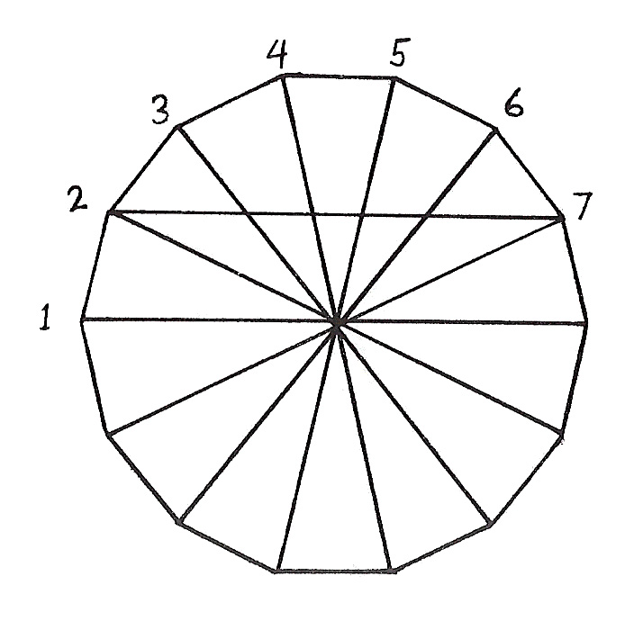
In the 7-zone star the relationship between the lengths of the radii and the line
S_{n}= 2S_{n - 1}+ S_{n - 2}- S_{n - 3}\label{eq:1}
or, for example,
283 = 2(126) + 56 - 25 \label{eq:equation4}
The first terms in the sequence are…1, 2, 5, 11, 25, 56, 126, 283, 636, 1429, 3211, 7215, 16212, 36428, 81853
\dfrac{11}{5}= 2.20000 \label{eq:equation5}
\dfrac{283}{126}= 2.24698 \label{eq:equation6}
\dfrac{7215}{3211}= 2.24696 \label{eq:equation7}
\dfrac{81853}{36428}= 2.24698 \label{eq:equation8}
Calculating the value from 10 place trigonometry tables
\dfrac{radius}{\overline{45}}= 2.24701 \label{eq:equation9}
The relationship between the radius and the line
S_{n}= S_{n - 1}+ 2S_{n - 2}- S_{n - 3}\label{eq:equation}
The more you examine properties of objects and phenomena, the more you find yourself presented with a few terms, usually simple, from a long series of terms. Often you cannot touch the terms which are farther or lower in the series, but you can define properties which they have. One gets the feeling of living in a container - one of an infinite number - to which are shunted objects and phenomena which have passed through one filter but can’t pass through another; a great process like that which takes place in a gravel yard, only we are unable to see gravel other than that of our own size but sense that it exists in endless different piles beyond - everything from sand to piles of planet sized boulders.
1 + \dfrac{1}{1 + \dfrac{1}{1 + \dfrac{1}{1 + \dots}}}\label{eq:equation2}
We can truncate the fraction anywhere and compute its value. The farther we carry it the closer it approximates the exact value;
T = \dfrac{\sqrt{5} + 1}{2}\label{eq:equation3}
Tau Power Series
| = | 0.2360680 | |
| = | 0.3819660 | |
| = | 0.6180340 | |
| = | 1.0000000 | |
| = | 1.6180340 | |
| = | 2.6180340 | |
| = | 4.2360680 | |
| = | 6.8541020 | |
| = | 11.0901699 | |
| = | 17.9442719 | |
| = | 29.0344418 |
: Tau Power Series
T^{n}= T^{n - 1}+ T^{n - 2}\label{eq:tau_power_series}
Pattern and Rules
If you begin with any two numbers and follow the rule, each term equals the sum of the two preceding terms, the ratio between consecutive terms approaches the divine proportion.
The first two terms of the Fibonacci numbers are 1, 1, and their proportion
\dfrac{F_7}{F_6}= 1.6250\label{eq:equation19}
\dfrac{F_{12}}{F_{11}}= 1.6180\label{eq:equation20}
Accompanying many simple polygons and patterns of polygons are series such as the Fibonacci, where the relationships between different terms approach the precise geometric relationships. The rules for forming the accompanying series are then clues for examining the structure of the pattern. And the relationships repeated in the pattern are clues for rules which give the process to form the pattern.
The perfection of the geometric form seems fragile. If we demand perfection to 7 decimal places, the thickness of a line spoils our form.
But the rules for the formation of the series which accompany the pattern are sturdy and simple. If mistakes are made in a sequence formed by the rules, the sequence heals itself after a few generations to again approach the precise form. This is seen in how quickly the Fibonacci series approaches
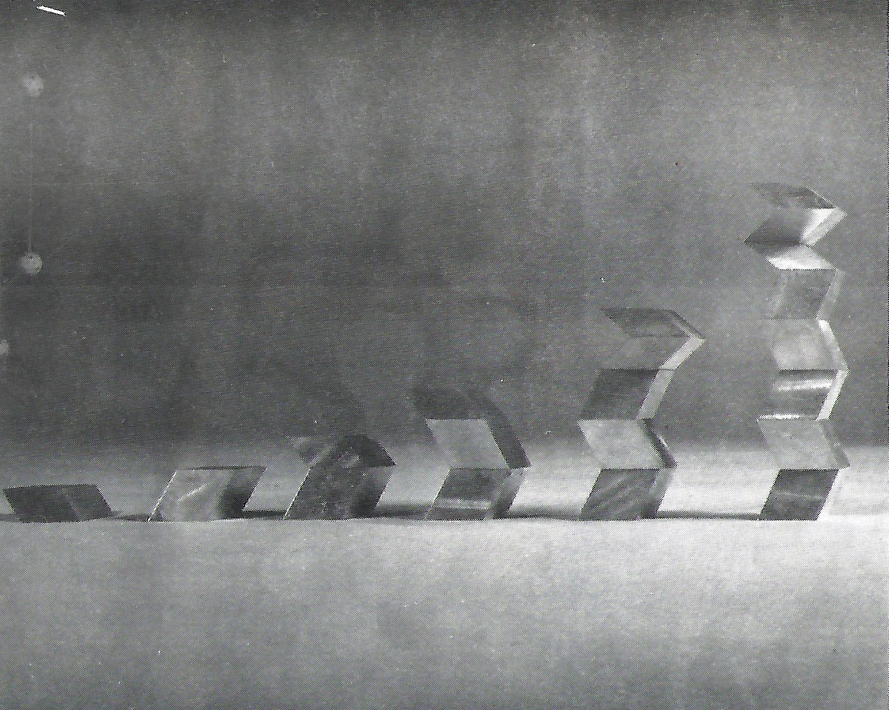
Stacks of six zone acute and obtuse cells. The widths of an acute cell and an obtuse cell are in the divine proportion. Therefore, a series of stacks can be built with each stack 1.6180339… times as tall as the one before it. The rule is that each stack is made by placing the two stacks that precede it on top of each other.
There are also numerous relationships involving the divine proportion among the altitudes of the parallelepiped cells formed with
The Fibonacci Numbers
| 1 | 89 | 10946 | 1346269 | ||||
| 1 | 144 | 17711 | 2178309 | ||||
| 2 | 233 | 28657 | 3524578 | ||||
| 3 | 377 | 46368 | 5702887 | ||||
| 5 | 610 | 75025 | 9227465 | ||||
| 8 | 987 | 121393 | 14930352 | ||||
| 13 | 1597 | 196418 | 24157817 | ||||
| 21 | 2584 | 317811 | 39088169 | ||||
| 34 | 4181 | 514229 | 63245986 | ||||
| 55 | 6765 | 832040 | 102334155 |
: Fibonacci Numbers
F_{n}= F_{n - 1}+ F_{n - 2}\label{eq:fib}
Coherence Proofs
In a structural system or any pattern the question arises; what is the pattern made of? What are the relationships between different elements of the pattern?
In a checkerboard pattern such as that shown in figure 9.11 all distances between neighboring intersections are the same. And the distance between two intersections of any line is simply a multiple of this base distance. This base distance then naturally becomes the unit for building the pattern.
In our pattern created by the star with five-fold symmetry, the situation is different. There are many different lengths between intersections. If the growth patterns follow simple rules such as those followed in forming the two-dimensional pattern of figure 9.21, then all distances between intersections can be expressed as simple sums of components whose lengths are equal to powers of the divine proportion times some constant. This is also true in three dimensions - the
s_{1}AT^{r_{1}}+ s_{2}AT^{r_{2}}+ \dots \ s_{n}AT^{r_{n}}\label{eq:equation11}
and the distance between two intersections on a
q_{1}BT^{t_{1}}+ q_{2}BT^{t_{2}}+ \dots \ q_{n}BT^{t_{n}}\label{eq:equation12}
The building blocks for our system are then a series of lengths related by the divine proportion. An
Two Dimensions
Definition 1
We call any particular polynomial of the form
s_{1}kT^{r_{1}}+ s_{2}kT^{r_{2}}+ \ldots \ s_{n}kT^{r_{n}}= f_{i}(kT) \label{eq:equation13}
We call the class of all such polynomials
f_{i}(kT) + f_{j}(kT) \in F(kT) \label{eq:equation14}
f_{i}(kT) - f_{j}(kT) \in F(kT) \label{eq:equation15}
(T^{n})f_{i}(kT) \in F(kT) \label{eq:equation16}
We are interested in the distances between intersections along the lines of certain sets of patterns.
Definition 2
A pattern is a number of extended lines which point in five different directions in one plane with at least one line pointing in each direction.
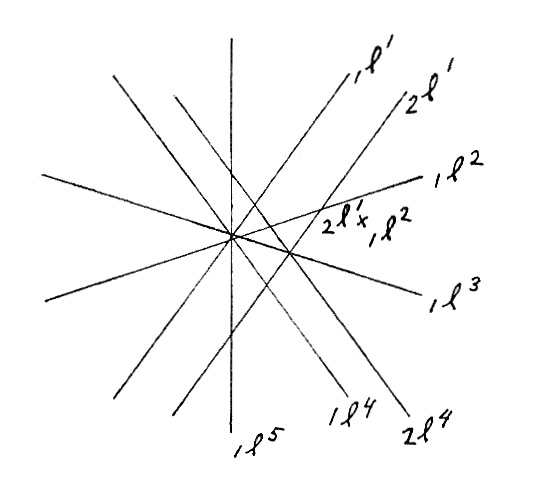
Definition 3
The lines are labeled; $$\begin
i^} & \
n & = 1, 2, 3, 4, 5 \
i & = 1, 2,\ldots \
\end$$
\dfrac{\pi}{5}, \dfrac{2\pi}{5}, \dfrac{3\pi}{5}, \dfrac{4\pi}{5}
Definition 4
An intersection is named by any two of the lines which intersect there, such as ```block-katex
j^}\times k^}\label
### Definition 5
If on a line all intervals between intersections are equal to different $`f_{i}(kT )`$, then the intersections “fit” each other.
An intersection fits a line if it fits all intersections on that line.
A line $`g^{l^{p}}`$ fits another line $`f^{l^{q}}`$ if the intersection $g^{l^{p}}\times
f^{l^{q}}$` fits all the intersections of `$f^{l^{q}}$.
A pattern fits if all the intersections on all the lines fit.
**Lemma 12.1**. *If on a line $`l^{n}`$ an intersection $`I_{n}`$ fits an intersection $`I_{m}`$ then $`I_{n}`$ fits all $`I_{o}`$ where $`I_{o}`$ fits $`I_{m}`$.*
**Lemma 12.2**. *Any $`i^{l^{m}}`$, $`j^{l^{n}}`$, $`h^{l^{p}}`$, $`m \neq n`$, $`n \neq p`$, $`p`$ form a triangle similar to $`T_{1}`$ or $`T_{2}`$*

### Definition 6
These triangles are called the Golden triangles because their sides are in the divine proportion.
**Lemma 12.3**. *If the two vertices of a Golden Triangle fit each other then all vertices fit each other.*
**Lemma 12.4**. *If a line $`j^{l^{m}}`$ fits a line $`h^{l^{n}}`$ and if all $`l^{n}`$ fit some line $`i^{l^{m}}`$ and if $`i^{l^{m}}`$ fits all $`l^{n}`$ without the line $`j^{l^{m}}`$, then, all intersections $`j^{l^{m}}\times l^{n}`$ fit $`j^{l^{m}}\times h^{l^{n}}`$ and the line $`j^{l^{m}}`$ fits all $`l^{n}`$.*
<figure id="fig:133">
<img src="content/images/fig-133.jpg" alt="Figure 133: " />
<figcaption aria-hidden="true">Figure 133: </figcaption>
</figure>
**Lemma 12.5**. *If $`j^{l^{m}}`$ fits $`h^{l^{n}}`$ then all $`l^{p}`$, $`p \neq m`$, $`n \times j^{l^{m}}`$ fit $`jlm \times hln`$ and if $`h^{l^{n}}`$ fits all $`l^{p}`$ without $`j^{l^{m}}`$ them $`j^{l^{m}}`$ fits all $`l^{p}`$.*
**Theorem 12.6**. *If a pattern fits and a line $`j^{l^{m}}`$ is added and $`j^{l^{m}}`$ fits some line $`j^{l^{n}}, n \neq m`$, then the new pattern including $`j^{l^{m}}`$ fits.*
*A pattern fits if all the intersections on all the lines fit. (Definition 5) To prove the new pattern fits we must prove all the new intersections fit the lines they are on.*
1. *There are no new intersections on the lines $`k^{l^{m}}, k \neq j`$, therefore all the intersections on these lines fit.*
2. *All the intersections $`j^{l^{m}}\times l^{n}`$ fit $`j^{l^{m}}\times h^{l^{m}}`$ and the line $`j^{l^{m}}\times h^{l^{m}}`$ and the line $`j^{l^{m}}`$ fits all $`l^{n}`$. (Lemma 4) Therefore all the intersections of the lines $`l^{n}`$ fit.*
3. *All the intersections $`l^{p, p \neq m,n}\times j^{l^{m}}`$ fit $j^{l^{m}}
\times h^{l^{n}}$`. (Lemma 5) Therefore, the intersections of line `$j^{l^{m}}$` fit `$j^{l^{m}}\times h^{l^{n}}$`. Therefore, the intersections fit on all the lines `$l^{m}$` (step 1) and `$j^{l^{m}}$` fits all `$l^{p, p \neq m,n}$` (Lemma 5) which means that all the intersections on all the lines `$l^{p,
p
\neq
m,n}$ fit and our theorem is thus proved.*
## Three Dimensions
### Definition 1
In three dimensions we have a pattern made up of the diameter lines through vertices and face midpoints of the icosahedron.
The lines through the vertices are the $`A`$ lines.
The lines through the face midpoints lines are $`B`$ lines.
There can be other lines parallel to the original 16 lines. They are given the name of the line they are parallel to.
We name a line $$\begin{aligned}
i^{A^{n^{1}}} & \\
n & = 1, 2, 3, 4, 5, 6 \\
i & = 1, 2, \ldots
\end{aligned}$$
$$\begin{aligned}
j^{B^{m^{1}}} & \\
m & = 1, 2, 3, 4, 5, 6, 7, 8, 9 ,10 \\
j & = 1, 2, \ldots
\end{aligned}$$
or generally
$$\begin{aligned}
h^{X^{p^{1}}_{i}} & \\
p & = 1, 2\ldots10 \\
h & = 1, 2, \ldots \\
X & = A, B
\end{aligned}$$
### Definition 2
All lines of a 3D pattern are connected directly or through other intersections to the original pattern of 16 lines.
### Definition 3
Intersections on $`A`$ lines “fit” if all the intervals between them can be expressed as polynomials ```block-katex
s_{1}AT^{r_{1}}+ s_{2}AT^{r_{2}}+ \dots \ s_{n}AT^{r_{n}}= f_{i}(AT)\label{eq:equation21}
Definition 4
Intersections on
s_BT^}+ s_BT^}+ \ldots \ s_BT^}= f_(BT)\label
$`s_{i},r_{i}=`$ integers and $`B =`$ an interval of length.

### Definition 5

```block-katex
B = \dfrac{\cos(\dfrac{\pi}{6})}{\cos(\dfrac{\pi}{10})}A\label{eq:equation23}
Definition 6
A 3D pattern “fits” if all the intersections on all the lines fit.
Definition 7
An
\dfrac{\pi - \theta - \phi}{2}\; \text{or}\; \dfrac{\pi - \theta - \phi}{2}\label{eq:equation24}
Definition 8
A
T^{A^{n}}
Lemma 12.7. There are five
Lemma 12.8. *The projection of the interval
= A \sin(\theta)\label
### Definition 9
*```block-katex
k = \sin(\theta) \; \text{ or }\; = 0.A\label{eq:equation26}
``` Unsure: What does 0.A resolve to? (if the interval is on the $`A`$ line perpendicular to the $`T`$ plane).*
**Lemma 12.9**. *The projection of the interval $`B`$ along any $`B`$ line onto a $`T`$ plane $$= B \sin(\dfrac{\pi - \theta + \phi}{2}) = k \; or \; = B \sin(\dfrac{\pi - \theta - \phi}
{2}= T^{-1_{k}})\label{eq:equation27}$$*
<figure id="fig:134">
<img src="content/images/fig-134.jpg" alt="Figure 134: " />
<figcaption aria-hidden="true">Figure 134: </figcaption>
</figure>
**Lemma 12.10**. *The projection onto any $`T`$ plane of any interval along any line $`k^{X^{r^{1}}_i}`$ between any two intersections which fit in the 3D pattern is a polynomial ```block-katex
s_{1}kT^{r_{1}}+ s_{2}kT^{r_{2}}+ \ldots + s_{n}kT^{r_{n}}= f_{i}(kT)\label{eq:equation17}
``` $$\begin{aligned}
s_{i},r_{i} & = \text{integers} \\
k = A \sin(\theta) & = B \sin(\dfrac{\pi - \theta + \phi}{2})
\end{aligned}$$*
**Lemma 12.11**. *The angles between the lines projected on a $`T`$ plane are ```block-katex
\dfrac{\pi}{5}, \dfrac{2\pi}{5}, \dfrac{3\pi}{5}, \dfrac{4\pi}{5}\label{eq:equation28}
```*
<figure id="fig:135">
<img src="content/images/fig-135.jpg" alt="Figure 135: " />
<figcaption aria-hidden="true">Figure 135: </figcaption>
</figure>
**Lemma 12.12**. *3D Patterns which fit project onto all $`T`$ planes 2-dimensional patterns which fit.*
**Lemma 12.13**. *All intervals between intersections of lines of the 3D pattern appear as intervals between intersections in the projections on some $`T`$ planes.*
*For an intersection ```block-katex
i^{X^{n^{l}}_{k}}\times i^{X^{m^{l}}_{j}}\label{eq:equation29}
``` not to appear as an intersection in the pattern projected on a $`T`$ plane, the intersecting lines must lie in one of the five perpendicular $`R`$ sections.*
*At most, two different lines intersect $`i^{X^{n^{l}}_{k}}`$. The two intersections ```block-katex
i^{X^{n^{l}}_{k}}\; \text{or}\; \; g^{X^{p^{l}}_{t}}
``` lie. Therefore, there is at least one $`T`$ plane in which both 3D intersections project as 2-dimensional intersections.*
**Lemma 12.14**. *If some pairs of intersections $$i^{X^{n^{l}}_{k}}\times h^{X^{m^{l}}_{j}}\; \text{and}\; \; i^{X^{n^{l}}_{k}}
\times g^{X^{p^{l}}_{f}}\label{eq:equation30}$$ did not fit in our 3D pattern, that is, we cannot find any polynomial $f_{1}(X_{k}
T)$` that equals the interval between them, then also for some `$T$` plane we cannot find a polynomial `$f_{i}(kT)$ which equals the interval between their projected intersections.*
**Lemma 12.15**. *Any misfits between intersections of the 3D pattern project as misfits between intersections on some $`T`$ plane. Therefore, a 3D pattern which projects on all $`T`$ planes as a 2D Pattern which fits is a 3D pattern which fits.*
**Theorem 12.16**. *If a 3D pattern fits and a new line is added $`k^{X^{n^{l}}_{i}}`$ which intersects and fits some other line $`h^{X^{n^{l}}_{j}}`$ then the new 3D pattern including $`k^{X^{n^{l}}_{i}}`$ fits.*
*Proof.* In each $`T`$ plane the projection of the line $`k^{X^{n^{l}}_{i}}`$ fits the projection of the line $`h^{X^{m^{l}}_{j}}`$. In each $`T`$ plane the projection of the 3D pattern without $`k^{X^{n^{l}}_{i}}`$ fits. Therefore, the projection is with the line $`k^{X^{n^{l}}_{i}}`$ fits on each $`T`$ plane and the theorem is proved. ◻
The coherence proof demonstrates that if one builds a structure using the $`A`$ and $`B`$ lines of the 31 zone star (the $`C`$ lines may be used only within the forms defined by the $`A`$ and $`B`$ lines) and always follows the rule that new parts are added at intersections of existing parts or at points along existing parts which can be reached by subdividing a large part into component small parts, then no matter how far or intricately one builds, two extensions of two entirely different limbs of the same structure can always be locked back together in a perfect fit with a combination of our simple parts.
We have shown that the intervals between intersections are all equal to certain polynomials in $`T`$. Because ```block-katex
T^{n}= T^{n - 1}+ T^{n - 2}\label{eq:equation31}
``` all the terms of any such polynomial can descend by subdivisions into a polynomial with only two terms- ```block-katex
f_{i}(AT) = rAT^{n}+ sAT^{n - 1}\label{eq:equation32}
``` There are many interesting side-lights to these investigations. One of which is that it is impossible to divide any one of our building blocks $`AT^{n}`$ into equal pieces.
There are much shorter proofs of the coherence of this system, but the short proofs don’t lead one through so many characteristics of the structure.
# Joints
We have associated the thirty-one zone star throughout with the icosahedron and the dodecahedron. It also fits perfectly with the three smaller regular polyhedra. The tetrahedron, the cube and the octahedron fit inside the icosahedron and the dodecahedron. Their vertices touch a vertex, an edge midpoint or a face midpoint of the larger figure. This regular match between large and small figure positions the smaller figure so that regular patterns on the large figure project inwards as regular patterns on the small figure. In each case, either five or ten small figures fit at once within the larger figure.[^4]
Each of the regular polyhedra is thus a convenient core from which to define the regular thirty-one zone star. The geometric regularities insure simplicity in the connections. Any one of the regular polyhedra can be used with the same pattern of flanges or holes on each of its faces as a connector for the thirty-one zone structural system.[^5]
<figure id="fig:136">
<img src="content/images/fig-136.jpg" alt="Figure 136: Tetrahedron" />
<figcaption aria-hidden="true">Figure 136: Tetrahedron</figcaption>
</figure>
<figure id="fig:137">
<img src="content/images/fig-137.jpg" alt="Figure 137: Tetrahedron Vertices" />
<figcaption aria-hidden="true">Figure 137: Tetrahedron Vertices</figcaption>
</figure>
<figure id="fig:138">
<img src="content/images/fig-138.jpg" alt="Figure 138: Cube" />
<figcaption aria-hidden="true">Figure 138: Cube</figcaption>
</figure>
<figure id="fig:139">
<img src="content/images/fig-139.jpg" alt="Figure 139: Cube Vertices" />
<figcaption aria-hidden="true">Figure 139: Cube Vertices</figcaption>
</figure>
<figure id="fig:140">
<img src="content/images/fig-140.jpg" alt="Figure 140: Octahedron" />
<figcaption aria-hidden="true">Figure 140: Octahedron</figcaption>
</figure>
<figure id="fig:141">
<img src="content/images/fig-141.jpg" alt="Figure 141: Octahedron Vertices" />
<figcaption aria-hidden="true">Figure 141: Octahedron Vertices</figcaption>
</figure>
<figure id="fig:142">
<img src="content/images/fig-142.jpg" alt="Figure 142: Dodecahedron" />
<figcaption aria-hidden="true">Figure 142: Dodecahedron</figcaption>
</figure>
<figure id="fig:143">
<img src="content/images/fig-143.jpg" alt="Figure 143: Dodecahedron Vertices" />
<figcaption aria-hidden="true">Figure 143: Dodecahedron Vertices</figcaption>
</figure>
<figure id="fig:144">
<img src="content/images/fig-144.jpg" alt="Figure 144: Icosahedron" />
<figcaption aria-hidden="true">Figure 144: Icosahedron</figcaption>
</figure>
<figure id="fig:145">
<img src="content/images/fig-145.jpg" alt="Figure 145: Icosahedron Vertices" />
<figcaption aria-hidden="true">Figure 145: Icosahedron Vertices</figcaption>
</figure>
# The Stars of Other Systems
In the design of a connector simplicity in one part may demand specialization and the establishment of hierarchies among other parts.
The sketches of a joint of an icosahedron show examples of different ways of joining the five edges of an icosahedron. The parts remain identical if they trade or share with each other at the joint.
<figure id="fig:146">
<img src="content/images/fig-146.jpg" alt="Figure 146: Sharing" />
<figcaption aria-hidden="true">Figure 146: Sharing</figcaption>
</figure>
<figure id="fig:147">
<img src="content/images/fig-147.jpg" alt="Figure 147: Trading" />
<figcaption aria-hidden="true">Figure 147: Trading</figcaption>
</figure>
When some parts dominate others, there is a hierarchy created and the parts must be differentiated. In our illustration, we show five edges of an icosahedron stacked on top of one another. With the icosahedron, it is possible to have both ends of each edge occupy similar positions, but this is not always true.
<figure id="fig:148">
<img src="content/images/fig-148.jpg" alt="Figure 148: Dominating" />
<figcaption aria-hidden="true">Figure 148: Dominating</figcaption>
</figure>
The creation of one hierarchy may create the need for more. For instance, if you wish to use a hierarchy of stacked edges to make a simple triangle, then you must also create a hierarchy between ends of the same edge. The two ends of the same edge have different ranks.
<figure id="fig:149">
<img src="content/images/fig-149.jpg" alt="Figure 149: Stacked Edges of a Triangle" />
<figcaption aria-hidden="true">Figure 149: Stacked Edges of a Triangle</figcaption>
</figure>
Very often we don’t have the structural members actually touching each other. Then we avoid the edges’ problem of sharing, trading or dominating—we push the entire problem on to the joint. The joint must accommodate all the connecting members, and it shouldn’t demand that they have elaborate ends or different kinds of ends. The joint must also be strong and inexpensive.
If the joint is a ball and the $`A`$, $`B`$ and $`C`$ connections are simply holes which the members screw into. All holes of the same type are identical, and the ends of all structural members are identical.
This is a wonderful feature because you can’t make mistakes—there are no right and wrong holes of a certain type. The joint shown in Figure [15.2](#fig:159){reference-type="ref" reference="fig:159"} has 12 threaded holes for the $`A`$ lines in the thirty-one zone system. Joints made this way are expensive, and the connectors at the end of the structural members are expensive. A common inexpensive connecting system is a joint made of multiple interconnecting flanges with the flattened ends of the structural members bolting against the flange of the joint. Joints made of flanges can be simple flat stampings that lock together or are welded together.
Flanges bring problems. What if you must connect two joints, and you find that once you bolt one end of your member to one joint it can’t bolt to the other because the flange is turned the wrong way? The specialization of a flat end and a flange has brought problems. The end of the structural member could be made to swivel. That is expensive. The joint could be made so that this problem never arises. Unfortunately, our second solution is not always possible. To make a thirty-one zone joint where each connection is a flat flange and which is impossible to put together incorrectly, you have to devise a pattern that passes through each connecting point only once and is regular (you can’t tell the pattern that surrounds a connection from the pattern that surrounds any other connection of the same type).
<figure id="fig:150">
<img src="content/images/fig-150.jpg" alt="Figure 150: Flanges of an icosahedron or dodecahedron" />
<figcaption aria-hidden="true">Figure 150: Flanges of an icosahedron or dodecahedron</figcaption>
</figure>
This is impossible to do in the case of the thirty-one zone star. You can make a flange joint for the thirty $`C`$ connections. The $`C`$ lines can have the specialization of flange orientation while still avoiding the clumsiness of having to arrange themselves in a hierarchy. The flanges are the edges of an icosahedron or a dodecahedron.
Three interlocking rectangles at right angles to each other form a flange joint for the 12 $`A`$ lines, 6 $`C`$ lines and 12 $`B`$ lines.
<figure id="fig:151">
<img src="content/images/fig-151.jpg" alt="Figure 151: Interlocking rectangles forming a flange joint" />
<figcaption aria-hidden="true">Figure 151: Interlocking rectangles forming a flange joint</figcaption>
</figure>
Note! These are three perpendicular $`R`$ sections.
There is a mistake proof flange joint for both $`A`$ and $`C`$ connections if one hierarchy is introduced. You must always orient the joint to suit the $`A`$ lines.
This joint is shown in the photo of the wooden model of the three intersecting planes.
<figure id="fig:152">
<img src="content/images/fig-152.jpg" alt="Figure 152: Model of intersecting planes" />
<figcaption aria-hidden="true">Figure 152: Model of intersecting planes</figcaption>
</figure>
Two of the flanges for the missing $`C`$ lines are added. This joint is completely regular until the addition of these $`C`$ flanges—they are not in the same plane as their neighboring $`A`$ flanges. We thus have two types and lose our regularity.
A good flange joint for the thirty-one zone star is made of six interlocking disks—five $`R`$ sections and one $`T`$ section.
<figure id="fig:153">
<img src="content/images/fig-153.jpg" alt="Figure 153: Six interlocking disks" />
<figcaption aria-hidden="true">Figure 153: Six interlocking disks</figcaption>
</figure>
<figure id="fig:154">
<img src="content/images/fig-154.jpg" alt="Figure 154: Vertices on a sphere" />
<figcaption aria-hidden="true">Figure 154: Vertices on a sphere</figcaption>
</figure>
This creates an irregular icosahedron which passes through each of the sixty-two connecting points and decides automatically the orientation of sixty of the flanges. The pole points of this figure are $`A`$ connections and one of the five intersecting $`R`$ sections must dominate the others to determine the flange orientation. This joint can have part or all of the $`R`$ sections in place depending on which connections are needed.
## Octet Truss
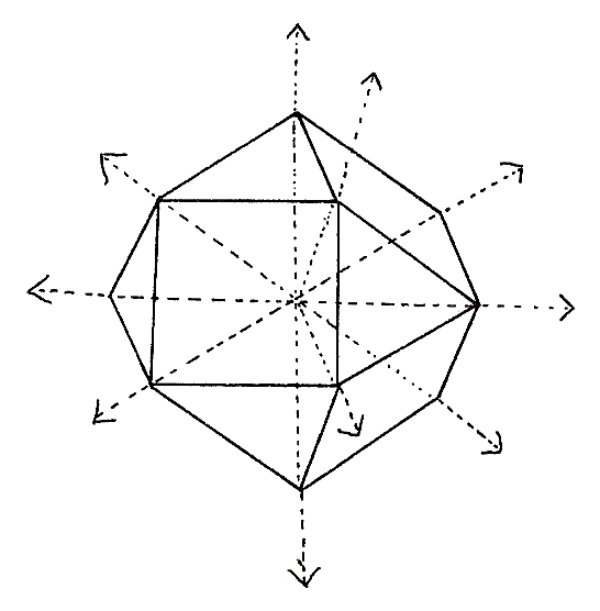
The widely used octet truss is based on the star that passes through the midpoints of the edges of a cube. (Or, equivalently, the midpoints of the edges of an octahedron, the midpoints of the faces of a rhombic dodecahedron, the vertices of a cuboctahedron.)
<figure id="fig:155">
<img src="content/images/fig-155.jpg" alt="Figure 155: Star for octet truss" />
<figcaption aria-hidden="true">Figure 155: Star for octet truss</figcaption>
</figure>
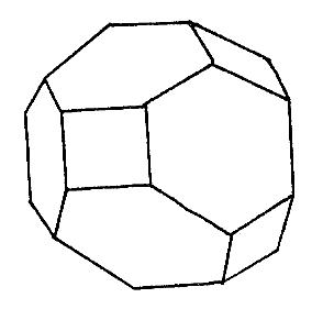
This is a singular star with four sections ($`A`$ sections in drawing) containing three lines at $`60\degree`$ to each other and three sections with two lines at right angles ($`B`$ sections). The zonohedron whose edges are parallel to the lines of the star is the truncated octahedron.
<figure id="fig:156">
<img src="content/images/fig-156.jpg" alt="Figure 156: Truncated Octahedron" />
<figcaption aria-hidden="true">Figure 156: Truncated Octahedron</figcaption>
</figure>
## The Mero Space Grid System
This system is based on the octet truss star plus three more zones which pass through the face midpoints of the cube which has the other lines passing through its edge midpoints. This singular star has three sections ($`B`$ sections) with four lines intersecting at $`45\degree`$ to each other, four sections ($`A`$ sections) with three lines at $`60\degree`$ to each other and six sections ($`C`$ sections) with two lines at $`90\degree`$ to each other.
<figure id="fig:157">
<img src="content/images/fig-157.jpg" alt="Figure 157: Star for MERO system" />
<figcaption aria-hidden="true">Figure 157: Star for MERO system</figcaption>
</figure>
The zonohedron associated with this star is the truncated cuboctahedron.
<figure id="fig:158">
<img src="content/images/fig-158.jpg" alt="Figure 158: Truncated Cubooctahedron" />
<figcaption aria-hidden="true">Figure 158: Truncated Cubooctahedron</figcaption>
</figure>
# Hardware
   
Lengths of $`A`$, $`B`$, and $`C`$ lines.
Structural members where $`A = 40''`$.
<figure id="fig:six_zone_joint">
<img src="content/images/fig-six-zone-joint.jpg" alt="Figure 159: Six Zone Joint Plan" />
<figcaption aria-hidden="true">Figure 159: Six Zone Joint Plan</figcaption>
</figure>
<figure id="fig:159">
<img src="content/images/fig-159.jpg" alt="Figure 160: Six Zone Joint" />
<figcaption aria-hidden="true">Figure 160: Six Zone Joint</figcaption>
</figure>
<figure id="fig:160">
<img src="content/images/fig-160.jpg" alt="Figure 161: Section for 1” pipe" />
<figcaption aria-hidden="true">Figure 161: Section for 1” pipe</figcaption>
</figure>
<figure id="fig:161">
<img src="content/images/fig-161.jpg" alt="Figure 162: Framework for Robert Ford residence." />
<figcaption aria-hidden="true">Figure 162: Framework for Robert Ford residence.</figcaption>
</figure>
$`A`$ lines = $`AT^{2}`$; base $`A = 40''`$
$`C`$ lines $`= CT^{2}`$ (see page 32)
<figure id="fig:162">
<img src="content/images/fig-162.jpg" alt="Figure 163: Zome Climber" />
<figcaption aria-hidden="true">Figure 163: Zome Climber</figcaption>
</figure>
$`A`$ lines $`= 40''`$ $`C`$ lines $`= 42''`$
# Bibliography
Baer, Steve - *The Dome Cookbook* - Lama foundation, New Mexico - 1968
Borrego, John - *Space Grid Structures (Skeletal Frameworks and Stressed-Skin Systems)* - MIT Press - Massachusetts - 1968
An exhaustive study of a few simple kinds of space grids with excellent illustrations of both the geometries and the hardware.
Courant and Robbins - *What is Mathematics? (An elementary approach to ideas and methods)* - Oxford University Press 1941 & 1953
A good book for anyone who thinks about curious and profound questions in mathematics. It has a good section on continued fractions and infinite series.
Coxeter, H. S. M. - *Regular Polytopes* - The MacMillan Co. New York - 1948 & 1963
This book has the most information about the regular polyhedra that I have seen. It is a difficult book for beginners. It has a good section on zonohedra. There are interesting historical remarks at the chapter ends.
Cundy and Rollett - *Mathematical Models* - Oxford at the Clarendon Press - 1951 & 1961
A good simple book on polyhedra and interesting mathematical models. The illustrations are the best that can be found.
Hilbert, David and S. Cohn-Vossen - *Geometry and the Imagination* - Chelsea Publishing Co. - New York - 1952
Many interesting and varied subjects are covered in this book. An excellent chapter on regular systems of points.
Hoggatt, Verner E. Jr, - *Fibonacci and Lucas Numbers* - Houghton Mifflin Co. - Boston - 1969
Short clear text. The best of the books on Fibonacci numbers.
Kowalewski, Dr. Gerhard - *Per Keplersche Korper und Andere Bauspiele* - K. F. Koehlers Antiquarium - Leipzig 1938
An account of the triacontahedron including the appearance of the divine proportion in its measurements, its breakdown into 20 parallelepipeds, the plaiting of its faces and ways of coloring its faces.
Ogilvy and Anderson - *Excursions in Number Theory* - Oxford University Press , New York - 1966
An excellent book on number theory with a lucid chapter about continued fractions.
Thompson, D’Arcy - *On Growth and Form* (Vol. 2) - Cambridge at the University Press - 1942 & 1963
Thompson discusses the divine proportion and the Fibonacci numbers and their appearance in nature.
Tyng, Anne Griswold - *Geometric Extensions of Consciousness* - English translation from ”Zodiac 19” magazine -
Filled with profound observations and important structural ideas.
Vorobyov, N. N. - *The Fibonacci Numbers* - D. C. Heath & Co. Boston - 1963
Short clear text.
Wachsmann, Konrad - *The Turning Point of Building* - Reinhold Publishing Corporation, New York - 1961
An excellent book about prefabrication, design, joints, panels and processes associated with the machine.
# Index
Accounting.
*See* Economic accounting
Anticipatory design science, 22
Anti-entropy, 101–102 *See also* Entropy
Areas. *See* Topology
Astronauts: all humans as, 56
Atomic energy, 129.
*See also* Energy Automation: of human biological processes, 54; and loss of jobs, 124
Automobiles: ownership of, 134
Bank wealth, 89
Behavioral sciences: in educational process, 26
Brain: as coordinating switchboard, 25; difference between mind and, 101; imitated by computer, 118
British Empire and the great pirates, 37–38
Categoryitis, 31
Children: as comprehensivists, 25–26 Circle. *See* Great circle Comprehension: defined, 77 Comprehensivity of Great Pirates, 34–35; Great Pirates abandoning their, 50–51; man forced to reestablish, 53
Computers: provide new impersonal problem solutions, 45; as superspecialist, 53; strategy combined with general systems theory and synergetics, 93–94; as imitation of human brain, 118; beginning of, 122; resolving ideological
dogmas, 138
Craftsmen: early specialized, 29; tools of, 122; in the industrial economy, 123
Cross-breeding: of world man, 131
Cybernetics: defined, 95
Darwin, Charles: theory of animate evolution, 47
Da Vinci, Leonardo, 35–36
Democracy, 92–93
Design: capability of early world men, 28–29; of spaceship Earth’s internal support systems, 59–60; of universal evolution, 111–112; revolution in, 134
Design science: anticipatory, governing yesterday’s naval mastery, 22
Divide and conquer: grand strategy of, 39
$`E = MC{^2}`$, 69, 96. *See also* Energy
Economic accounting: by great pirates, 94–95; synergy in, 103; need for realistic, 112
Educational task: to allow physical and metaphysical success, 130
Einstein, Albert: formula $`E = MC{^2}`$, 45, 69, 96; definition of physical universe, 70; reassess universe, 97
Electromagnetic spectrum: great pirates’ first use of, 43–44; effecting human evolution, 110 Energy: impounding of sun’s radiant, 58, 59, 93; generalized law of, 73; savings as fossil fuels, 94, 129; in synergetics, 95; finite, 96; harnessing of, 129; atomic exploitation of, 129
Entropy: energy systems eventually run down, 46; assumed universe subject to, 96; wealth as antientropy, 101
Environment: early society inability to cope with, 26; evolution synergeticaily produced, 103–104; changes in physical, 110
Euler, Leonhard, 81
Evolution: success of human dependent on mastering metaphysical, 46; design and patterns in, 49, 54, 111–112; man’s feeling about, 53–54; inexorable, 55; our present position in, 65–66; effected by electromagnetic spectrum, 110; comprehending phases of, 127
Experiences: to extract generalized principles, 62; is finite, 70
Exploitation: of atomic energy, 129; of fossil fuels, 129. *See also* Energy
Extinction, 48
Failures: humanity’s, 24–25 Fellowships, 125
Forecasting, 22
Fossil fuel: energy savings account, 94, 128; expending of, 129. *See also* Energy
Generalized principles: minds discovering, 21; extracted from human experience, 61–62; first was leverage, 63; surviving with, 118; inventively employed only through mind, 127
Genera! systems theory: as tool of high intellectual advantage, 67, 70–71; combined with computer strategy and synergetics, 95
Geodesic lines, 76
GI Bill, 115
Gold: demand system inadequate, 88–98; used by Great Pirates for trading, 90
Grand strategy: divide and conquer, 39; organizing our, 65.
*See also* Strategy
Great circle: defined, 76
Great Pirates: as sea mastering people, 34; feared bright people, 35; use of logistics by, 37; and British Empire, 37–38; use of local strong man as king by, 39; tutoring of bright specialists by, 40; in world competition, 41, 43; becoming extinct, 44, 50; rules of accounting still used, 45
Gross national product: estimate for 1970, 108–109
Growth: physical and metaphysical, 61
“Have-nots” struggle with “haves” produces war, 87
“Haves”: struggle with “have-nots” produces war, 87
Heisenberg, Werner: principle of indeterminism, 72
Human beings, as astronauts, 56; will be free, 111; employing real wealth, 124; characteristics in Mexico, 132. *See also* Man
Humanity: exists in poverty, 23–24; on Earth’s surface, 27; extinction of, 49; place in evolution of, 66; function of, in universe, 83–84; and standard of living of, 102–103
Ideologies: political, 48; resolving dangerous dogmas of, 138
Indeterminism: Heisenberg’s principle of, 72
India: population problems in, 113 Industrialization: demonstration of world, 104
Industry: tooling of, 22, 116, 122, 133; production increased by world wars, 116; craftsmen in the economy, 123. *See also* Tools
Information: multiplies wealth, 104–105 Initiative, 45
Intellect: as humans’ supreme faculty, 60–61; frees man of special case superstition, 63; use of as man’s function in universe, 99
International Monetary Fund: 1967 deliberations of, 88
Invention, 134
Inventory: of variables in problem solving, 67–68
Jobs: loss of in automation, 124
King: as great pirate’s local strong man, 39, 40
Law of conservation of energy: defined, 98. *See also* Energy
Learning: always increases, 99; man’s past, 131; industrial retooling revolution, 133
Lesser circle: defined, 76
Leverage: first generalized principle, 63. *See also* Generalized principles
Life: as synergetic, 79–80; hypothetical development of support systems in, 107–108
Lincoln, Abraham, 45–46
Lines, 81. *See also* Topology
Machine: spaceship Earth as, 59–60 Macrocosm: as universe outside the system, 70
Malthus, Thomas, 47
Man: utterly helpless as newborn, 61;
as adaptable organism, 118–119.
*See also* Human beings
Mass production: and mass consumption, 123
Mathematics: improved by advent of zero, 36. *See also* Topology
Metals: not destroyed in war, 117 Metaphysical: initiative confused between religion and politics, 45; masters the physical, 46; experiences not included in physical universe, 68; defies “closed systems” analysis, 69; in synergetics, 95; need for, in educational task, 130
Mexico: human characteristics in, 132 Michelangelo, 35–36
Microcosm: universe inside the system, 70
Mind: comprehends general principles, 24, 127, 128; difference between brain and, 101; fellowships of, 125
Money: as bank wealth, 89.
*See also* Wealth
Moon gravity: as income wealth, 94 More-with-less: and generalized principles of, 63
Myth: of wealth as money, 114;
of population explosion, 136 Natural laws: and Great Pirates, 34.
*See also* Generalized principles Navies: and Great Pirates, 38 Negatives: yesterday’s, realized, 24 North America: early crossbreeding men in, 131
Photosynthesis: impounds sun’s energy, 59
Pirates. *See* Great Pirates
Planck, Max, 97
Planners: more comprehensive than other professions, 67
Points. *See* Topology
Politicians: local, asked to make world work, 51.
*See also* Ideologies
Pollution: as survival problem, 85 “Poluto”: as new name for planet, 85 Population: problems in India, 113;
explosion in as myth, 136 Poverty: humanity existing in, 23–24 Principles. *See* Generalized principles Problem solving: by yesterday’s
contrivings, 21
Resources: of Earth unevenly distributed, 29; no longer integratable, 52; unique materials made “on order,” 106
Revolution: design and invention, 134
Safety factor: in man’s evolution, 111–112
Schools: beginning of, 41.
*See also* Specialization; Strategy Second law of thermodynamics, 46 Senses: Great Pirates relying on, 43 Ships: logistics for production and maintenance, 37. *See also* Vessels
Slavery: of specialist expert, 41; human, 107
Sovereignties: claim on humans in, 37–38; categoryitis in, 31
Spaceship Earth: present condition of, 121
Specialist: computer as super, 53 Specialization: society operates on theory of, 25; early leaders who developed, 26, 30, 33; intellectual beginning of schools, 41–42; specialist as slave, 41; over causing extinction, 48, 49; scientific, applied toward weaponry, 52–53
Speed of light: discovery of, 97 Spending: regarding energy is obsolete, 98
Spoken word: as first industrial tool, 122
Strategy: secret and anticipatory, of Great Pirates, 35; comprehensive of naval war colleges, 37
Structures: industrial tool enclosing, 116–117
Students: comprehend elimination of war, 134
Sun: radiation as income wealth, 58, 94. *See also* Energy
Survival: physical and metaphysical, 61; potentials increased by intellect, 63
Sword: powerful men of, 26.
*See also* Great Pirates
Synergetics. *See* Synergy
Synergy: defined, 78, 95; defines universal evolution, 79; combined with computer strategy and general systems theory, 95; wealth develops interest through, 102; in economic accounting, 103; in humanity escaping from local identity, 106
System: universe as biggest, 68; thought is, 72; first subdivision of universe, 71, 83;
variables in evolution, 83
Technologies: as substitute after war, 117
Telford, Thomas: as Great Pirates’ specialist, 37
Thinking: long-distance future of, 22; in terms of whole, 67; as a system, 72; dismissal of irrelevancy in, 76–77; tackling problems with, 83; humans free to, 126.
*See also* Intellect; Mind
Time: as relative, 135
Tools: industrial, 116; externalizations of integral functions, 117; craft and industrial extinctions, 122; spoken word, 122
Topology: mathematics of comprehension, 77; discovered by Euler, 81; patterns of lines, points and areas, 80–81. *See also* Geodesic lines; Great circle; Lesser circle
Underlying order in randomness, 74–75 Universe: as biggest system, 68, 96; physical defined by scientists, 68–69, 70, 72, 97; subdivision, 71; generalized law of energy conservation in, 73; defined by synergy, 79; humanity’s function in, 83, 112
Van Allen belts, 58
Variables: inventorying of and
problem solving in, 67
Vectorial geometry: mathematics
of comprehension, 75–80
Vessels: use of, in venturing, 28
War: beginning of the great class, 47–48, 87; as age-old lethal formula of ignorant men, 52; as taking priority over real problems, 87; students comprehend elimination of, 134
Water: desalinization of, as problem solution, 85–86. Pollution
Wealth: generated by integrating resources, 29; as a safety factor, 61; defined, 88, 93; irreversible in evolutionary processes, 91; society’s real, 91, 94,124; income is sun radiation and moon gravity, 94; as anti-entropy, 101; can only increase, 101,105; common, of humanity, 105; of the U.S., 108; of know-how produced by GI Bill. 115
Weaponry: scientific specialization applied toward, 52
Wholes: thinking in terms of, 67; systems in synergy, 78. *See also* Systems
World: and first seafarers, 28; sea ventures thought in terms of, 30; asking local politicians to make it work, 51; defined, 104, 119; veterans returning from World War II, 115; increase industrial production in, 115–116; cross-breeding in, 131-132
# Bibliography
Brown, William Henry. 1935. *The Plant Kingdom: A Textbook of General Botany*. Boston: Ginn; company.
Cundy, H. Martyn, and A. P. Rollett. 1961. *Mathematical Models*. 2d ed. Oxford: Clarendon Press.
[^1]: See definition of singular star - Figure [2.13](#fig:21){reference-type="ref" reference="fig:21"}
[^2]: See Section [11.2](#sec:pattern-and-rules){reference-type="ref" reference="sec:pattern-and-rules"}
[^3]: See Critical Constants [7](#ch:critical-constants){reference-type="ref" reference="ch:critical-constants"} and Hardware [15](#ch:hardware){reference-type="ref" reference="ch:hardware"}.
[^4]: See illustrations in Cundy and Rollet’s ([Cundy and Rollett 1961](#ref-Cundy:1961wk)).
[^5]: Note! In the case of the thirty-one zone pattern projected on the octahedron, four of the faces have a left-handed pattern. The drawing and the photo are of patterns with different handedness.
# eBook Formats
- [epub](zome-primer.epub)
- [kfx](zome-primer.kfx)
- [mobi](zome-primer.mobi)
- [pdf](zome-primer.pdf)